REPORT (2012)

Evaluation for water gauge stations in GRAPHS

Summary evaluation in MAP

Flood forecasts hydrographs in GRAPHS

Flood REPORTS (only in czech)

Evaluation of Real-time Flood Forecasts in the Czech Republic 2002-2012

J. DAŇHELKA (1) AND T. VLASÁK (2)
(1) Czech Hydrometeorological Institute, Na Sabatce 2050/17, 143 06 Praha, Czech Republic jan.danhelkaADchmi.cz
(2) Czech Hydrometeorological Institute, Antala Staska 1177/32, 370 07 Ceske Budejovice, Czech Republic tomas.vlasakADchmi.cz

INTRODUCTION

Operational flood forecasting has developed significantly in many countries since the 1990s. Hydrological services mostly use conceptual hydrological models to provide short-term (typically 2- to 3-day) deterministic flow forecasts, while for longer lead times probabilistic (ensemble) forecasts are applied. Paradoxically, the evaluation of the real-time forecast is easier for probabilistic forecasts (using the Brier score or ranked probability score) while no single objective criterion exists to evaluate the success rate of the whole forecasted hydrograph.

Deterministic real-time flow forecasts are usually evaluated after the flood with the aim of assessing the effect of various sources of uncertainty (for more information on uncertainty in hydrological forecasting see Maskey 2004, Krzysztofowicz 1999) although it is a very complicated issue. However, forecast users mostly do not recognize the particular steps of the process of flow forecasting, and thus do not distinguish between sources and reasons for the final “imprecision” of the forecast. In this work, we have applied the user’s point of view and we have simply evaluated the success rate of flow forecasts without identifying the factors affecting the process of its development.

METHODS

The Czech Hydrometeorological Institute (CHMI) is responsible for flood forecasting in the Czech Republic. CHMI operates the AquaLog flood forecasting system for the rive Elbe basin and the HYDROG flood forecasting system for the river Danube and the rive Odra basins. Both systems are used to provide 48h lead time deterministic forecasts for more than one hundred water gauging sites on a daily basis (or more often during floods). In this study, archived forecasts covering the period from 2002 to 2010 were analyzed. Unfortunately, the archive was not systematic over the whole period, resulting in gaps in the time series for some of the evaluated sites.

2.1 Flow forecast evaluation criteria

The Nash-Sutcliffe criterion (eq. 1) is generally applied as a basic measure of model performance in cases of long-term simulation. But its application to a single forecasted hydrograph is not appropriate because of small datasets (in our case, 48 values of hourly forecasts) and changes in the leading processes and factors that affect the forecast error by the lead time. It also cannot be used to evaluate more forecasts, because they usually overlap and/or make discontinuous time series. As a result, there is no single objective criterion generally accepted as a standard measure of real-time forecast performance and a visual check remains the most important evaluation technique. However, as discussed during the IAHS Workshop on “Expert judgement vs. statistical goodness-of-fit for hydrological model evaluation: Results of experiment” during the XXV IUGG 2011 General Assembly, some pattern-matching criteria provide reasonable performance in evaluating high flows (see the report at http://www.stahy.org). We especially draw attention to the procedure “Series Distance” proposed by Ehret and Zehe (2011).

Flood forecasts are the basis for decision-making, which in reality is mostly threshold based. Therefore in this article, we have simplified the forecast to a single value (peak flow, total flow volume, threshold exceedance) to which the following evaluation criteria were applied:

• Peak flow relative difference
• Total flow volume relative difference
• Hit Rate (HR)
• False Alarm Ratio (FAR)
• Frequency Bias (FB)
• Critical Success Index (CSI)

Criteria 3 to 6 are based on the concept of categorical evaluation as used by Morris (1988). Evaluation is based on defining an event of a flood as peak flow over the given threshold (flood risk stage) and a simple contingency table (fig. 1) defining four possible categories - Hit, False Alarm, Miss, and Correct Rejection.

		event forecasted
		YES	NO
event observed	YES	HIT (H)	MISS (M)
	NO	False Alarm (FA)	Correct Rejection (CR)

Fig. 1 Contingency table

When data were split into the described categories, various simple statistics could be calculated (Stanski et al., 1989). Hit Rate (HR) or Probability of Detection describes the ratio of successfully forecasted events and all observed events (eq. 2). HR values range from 0 (the worst) to 1 (the best), however, good values may be on account of a high False Alarm Ratio (eq. 2). Frequency Bias (eq. 3) describes the ratio of forecasted and observed events. FB value >1 indicates over-forecasting (events are forecasted more often than they occur), value < 1 indicates under-forecasting. Critical Success Index (eq. 4) is the most complete of the selected measures, it ranges from 0 to 1 (the best).

HR = H / (H+M) [1]
FAR = FA / (H +F) [2]
FB = (H + FA) / (H + M) [3]
CSI = H /(H + FA + M) [4]

The evaluation was performed for a subset of archived forecasts for which threshold exceedance was forecasted or observed within the 48h period of its lead time. If the observed flow was already above the threshold at the time of forecast issue, the forecast was not included in evaluation.

Thresholds were defined according to Czech flood management practice as three thresholds of flood risk stages (1 - flood watch, 2 - flood alert, 3 - flooding). Flood watch usually corresponds to a 1- to 5-year flow return period. The application of the flood watch threshold provided subsets of 10 to 120 forecasts at particular sites. In addition, for some analysis we also used flow return periods of 1-, 2-, 5- and 10-year floods.

The reliable lead time of forecasts was evaluated according to Corby and Lawrence (2002), using an average lead time of “hits” and by computing the Nash-Sutcliffe coefficient (eq. 5) separately for each of the time steps within the forecast lead time.
,[5]
where S is forecasted flow, O is observed flow, and i indicates a particular time step.

RESULTS

Unless indicated otherwise, the presented results are based on an evaluation of exceedances of the “flood watch” threshold.

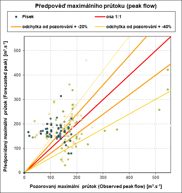
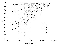
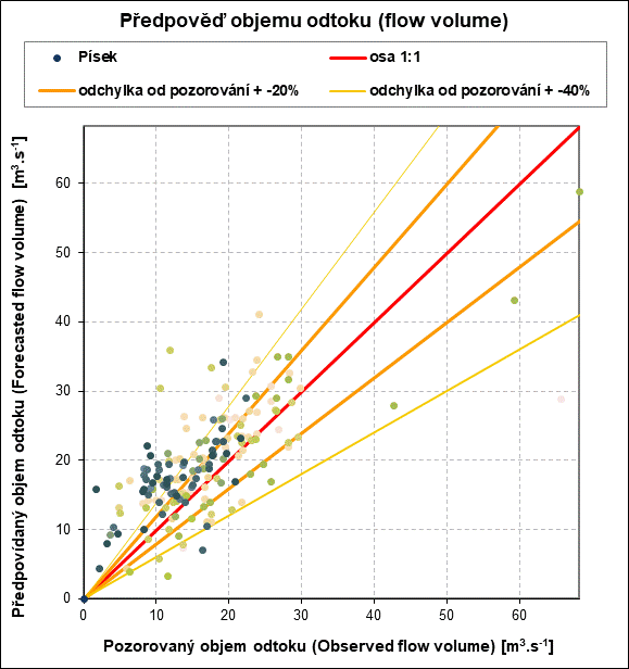Fig. 2 Scatter plots of the flow volume and peak flow forecast errors for the river Otava in Písek (2,914 km2)

Results generally indicate that about one-third of the forecasts ranked as hits, one-third as misses, and one-third as false alarms. The average hit rate was 0.34 (miss rate = 0.33, false alarm rate = 0.32, CSI = 0.34). However, large differences exist between the sites. While differences in the proportion of H, FA and M seem to follow a regional pattern (Fig. 3, 4, 6, 9 and 10), differences in CSI (Fig. 7) and the reliable lead time (Fig. 8) reflect differences in the time of runoff concentration between small mountainous basins and larger rivers. Differences in the reliable lead time were expected because the impact of a quantitative precipitation forecast increases rapidly for small basins, while for large or slowly reacting (e.g. the river Lužnice) basins forecasts depend more on observed data (precipitation and discharges upstream) and thus remain less uncertain.

The observed regional pattern (the difference between southwest on the one hand, and the north on the other hand) cannot be objectively explained in any simple terms. However, a reason could be forecasters’ different strategies, since a pattern of a higher FA ratio (and other criteria) reflects the area of responsibility of the Plzeň and České Budějovice Regional Offices together with a different fit of parameter sets due to different basin characteristics.

Forecasts of flow volume show a higher percentage of successful forecasts than those of peak flow. That could be explained by the used interface between the meteorological (NWP) and hydrological models. QPF inputs to hydrological model as 6h accumulated areal average (for areas of approximately 1,000 to 2,000 km2) to avoid the error of the localization of spatially limited precipitation (convective storms). Peak flow forecasts are, naturally, more sensitive to such smoothing out of rainfall intensity in space and time.

Fig. 3 H-M-FA proportion	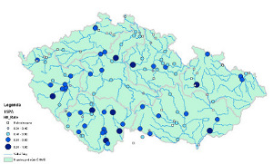Fig. 4 Hit rate	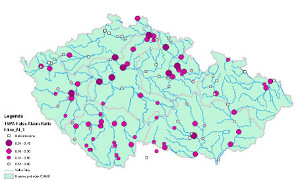Fig. 5 False Alarm Ratio
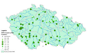Fig. 6 Frequency Bias	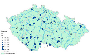Fig. 7 Critical Success Index	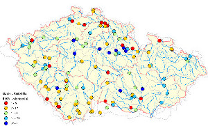Fig. 8 Lead time (h) of NS falling bellow 0.5
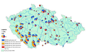Fig. 9 Total flow volume forecast performance	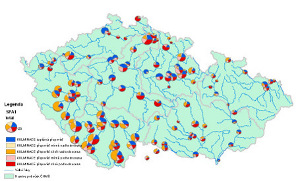Fig. 10 Peak flow forecast performance

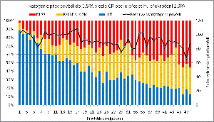
An important factor of flood forecasting is an effective lead time of the forecast, which determines the flood manager’s possibilities to prepare for flood and manage flood control activities. As we have demonstrated, the overall forecast performance increases with the basin’s time of runoff concentration. The assumption that forecast performance decreases with lead time was proved by the evaluation of the H-M-FA proportion, dependent on lead time of the forecasted (for H and FA) or observed (M) threshold (flood watch) exceedance (Fig. 11). Evaluation was performed over the whole dataset of all forecast in all profiles to ensure a sufficient number of events for statistics.

Figure 11 documents the fast decrease in the hit proportion during the first 18 hours of the forecast. That corresponded well with the typical time of runoff concentration in headwater basins having areas of up to several hundreds of km2. The H-M-FA proportion then remained stable for another 30 hours of the forecasting interval. However, HR decreased to 10 to 20% only, while it was 50 to 70% during the first hours of the forecast.

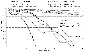
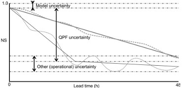
Similar results were obtained by lead time dependent Nash-Sutcliffe (NS) computed for each forecasting site (Fig. 12 and 13). While for slowly reacting larger rives NS remained more or less stable and very close to 1 during the whole forecasting interval, for small rivers the NS value decreased typically after 6 to 18 hours. Figure 12 illustrates NS for five selected sites with different upstream basin areas. For all sites, NS computed from a set of events of flood watch exceedance is compared with NS based on all issued forecasts. Expectably, flood based NS values were lower due to a higher impact of QPF uncertainty during the flood events in comparison with normal or low flow conditions.

We observed two types of the behaviour of NS decrease with lead time. Larger rivers exhibited a more or less stable decreasing trend over the forecast’s whole interval. Surprisingly, a large number of small streams had a similar behaviour but with a steeper slope of the trend line. Other small streams usually showed a fast decrease followed by oscillations with a flat trend (Fig. 14). Assuming that the difference of the 1st hour NS from 1 is due to model uncertainty (including parameters, model structure, and observed data error) and that the oscillation with no trend was due to other random sources (operational uncertainty as defined by Krzystofowicz, 1999), then we could estimate the proportions of different sources of uncertainty. Based on such assumption we have estimated that QPF was responsible, on average, for 65% (median = 71%) of the total forecast uncertainty (error) for basins with a size of < 500km2. Model uncertainty estimation was 7% on average (3% median), operational uncertainty probably accounted for 29% on average (22% median).

Fig. 12 Lead time dependent Nash-Sutcliffe criterion for selected forecasting sites for all forecasts and forecasts of flood watch exceedance.

Fig. 13 NS values for dependence of selected lead times on the basin area. .

Fig. 14 Lead time dependent Nash-Sutcliffe criterion for selected forecasting sites for all forecasts and forecasts of flood watch exceedance

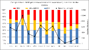
The H-M-FA proportion varies with the selected threshold (flood risk stage) as well as in time. However, the variation between different applied thresholds was surprisingly small (Fig. 15). This suggests a stable reliability of forecasts for the magnitude of flow between the flood watch and flooding stages that correspond to approximately 1- to 20-year return periods. From the user’s point of view it means that forecasts of a high flood stage (flooding) are as trustable as forecasts of low flood stages.

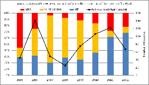
No trend in the H-M-FA proportion during the analyzed period from 2002 to 2010 (Fig. 16) was found. Differences between particular calendar years could be explained by the different predictability of the flood events that dominated selected years. For example, the slightly more successful years of 2003 and 2006 were dominated by spring snow melting floods due to a heavy snowpack and temperature rise, with a limited impact of liquid precipitation; such conditions are generally easier to predict by NWP.

The variability of the annual course of the H-M-FA proportion (Fig. 17) was caused by different numbers of events between calendar months on the one hand, and different typical seasonal flood causes on the other hand. April is a season of frequent weather changes in Central Europe, with a large number of frontal systems passing from the Atlantic. However, precipitation occurs mainly in connection with convection associated with fronts, which makes it difficult to predict precisely in terms of intensity, space and time for NWP. This may be the reason of the large number of FA in April.

High values of M occurred in February and from October to December. These were months with the smallest number of evaluated events, which may have skewed the results. In addition, results for October to December may have been affected by early snowfall and the hydrological model concept and calibration. The AquaLog system uses SAC-SMA for rainfall-runoff modelling. SAC-SMA (Burnash et al., 1973) does not recognize interception as a separate process, but its effect is partly included in the Upper Zone Tension Water (UZTW) storage parameter, which remains stable during the year. However, due to the vegetation cycle, interception and evapotranspiration decrease significantly in October to December, which may result in an overestimation of the initial loss in UZTW and, consequently, in an underestimation of runoff.

Fig. 15 The H-M-FA proportion for different thresholds of flow

Fig. 16 Inter-annual variation of the H-M-FA proportion (for the flood watch stage)

Fig. 17 Annual variation of the H-M-FA proportion (for the flood watch stage)

CONCLUSIONS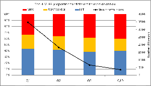

The real time forecasts were evaluated with the aim of identifying the performance of the whole forecasting chain towards an indication of flood stage exceedances at particular forecasting sites as supporting information for forecast users, especially flood managers. Results thus represent the predictability of “extreme events”, which is probably lower than for the whole set of forecasts.

Not only do we find the expected spatial differences in performance between small headwater basins and large downstream rivers (which proves the dominance of the QPF effect over the hydrological forecast success rate), but this pattern is, for some of the evaluation criteria, obscured by the regional pattern that copies the areas of responsibility of the CHMI’s Regional Forecasting Offices, indicating the impact of the forecasting strategy. The higher tolerance of FA in the southwest may be the effect of the 2002 flood experience and the common understanding established between forecasters and regional authorities on the preferred forecasting strategy.

Evaluation results serve as supplementary information for the interpretation by their user on the one hand, and as feedback for forecasters for the further development and enhancement of the forecasting system and procedures. From the point of view of a forecaster’s feedback, our results do not imply direct consequences in terms of model calibration changes (except for the effect of vegetation in the autumn and winter seasons) but they point to the issue of forecasters’ strategy as a determinative factor. The forecaster’s strategy affects forecasts trough the change of QPF input (based on meteorological forecasters’ guess) and interactive work with the model (change of initial conditions and parameters according to the current situation). Our recommendation is to define a common forecasting strategy for all Regional Forecasting Offices. The strategy itself should be discussed with flood managers to reflect their preferences as regards the acceptable number of misses and false alarms.

REFERENCES

• Burnash, R. J. C., Ferral, R.L. & McGuire R. A. (1973): A generalized streamflow simulation system - Conceptual modeling for digital computers, Technical Report, Joint Federal and State River Forecast Center, U.S. National Weather Service and California Department of Water Resources, Sacramento, USA.
• Corby, R. J. & Lawrence, W. E. (2002) A Categorical Flood Forecast Verification System for Southern Region RFC River Forecasts, NOAA Technical Memorandum NWS SR-212, Fort Worth, USA. Available at: http://www.srh.noaa.gov/ssd/techmemo/sr220.pdf
• Ehret, U. & Zehe, E. (2011) Series distance – an intuitive metric to quantify hydrograph similarity in terms of occurrence, amplitude and timing of hydrological events, Hydrol. Earth Syst. Sci., 15, 877–896.
• Krzystofowitcz, R. (1999) Bayesian Theory of probabilistic forecasting via deterministic hydrologic model, Water Resources Research, 35(9), 2739-2750.
• Maskey, S. (2004) Modelling Uncertainty in Flood Forecasting Systems, Taylor&Francis, London, UK.
• Morris, D. G. (1988) A Categorical, Event Oriented, Flood Forecast System for National Weather Service Hydrology, NOAA Technical Memorandum NWS HYDRO-43, Silver Springs, USA
• Stanski, H. R., Wilson, L. J. & Burrows, W. R. (1989) Survey of common verification methods in meteorology, WMO, World Weather Watch Report No. 8 (TD No. 358).