ANNEX I

DETAILED SPECIFICATION OF THE PRESENTED AIR POLLUTION MAPS

The spatial maps are based on the results of measurements in individual localities and they are created with the use and combination of various information (Chapter XII). The uncertainties of individual maps depend particularly on the density of measuring stations and the equivalent coverage across the CR territory, on the uncertainties of individual measurements, inputs to models, model calculations and the used method of the construction of the spatial maps. The greatest uncertainty of the maps is in the vicinity of the measuring stations. In spite of rather high uncertainties of some of the maps, these maps can be used for ambient air quality evaluation. It is necessary to take into account the uncertainties of the maps when interpreting them.
The following paragraphs present the background material used in the construction of air pollution maps for the year 2013, and the specification of individual maps presented in this yearbook.

1. The used data

1. Measured air pollution data: Annual characteristics of the measured data from the ISKO database are used.
2. Outputs of dispersion models: Outputs of the following models are used:
   SYMOS – Gaussian model, resolution 2x2 km, year 2012;
   CHIMERE – Eulerian model, resolution 7x7 km, year 2009;
   CAMx – Eulerian model, resolution 9x9 km, year 2009;
   EMEP – Eulerian model, resolution 50x50 km, year 2011 (PM₁₀), and 2012 (benzo[a]pyrene).
   The individual models used the latest outputs available whenever during the work on this yearbook.
3. Emissions from traffic: resolution 1x1 km, source: emission database REZZO 4 (year 2012).
4. Altitude: resolution 1x1 km, source: ZABAGED, Office for Surveying and Mapping.
    

2. The estimate of uncertainty

The estimate of uncertainty of the respective map used the cross-validation method, see Horálek et al. (2007). The estimate of concentrations in the measuring sites is produced always by withholding the given measurement using other data and thus creating the objective estimate of the quality of the map beyond the measuring site. This procedure was used repeatedly for all measuring sites. The estimated values were compared with the measured values with the use of the root-mean-square error (RMSE), or the relative root-mean-square error (RRMSE):
 

                 

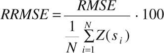
where

        Z(s_i)  is the measured value of the concentration in the i-th point,
          is the estimate in the i-th point using other data,
        N       is the number of measuring stations.

Due to computation reasons, the estimate of the uncertainty was calculated only for the interpolation of residual; the total uncertainty of the map is therefore slightly higher. It is also necessary to mention the fact that this is the mean uncertainty of the whole map, the spatial distribution of uncertainty was not estimated.

3. Parameters of individual maps

The following tables present the supplementary quantities used in the linear regression model and their parameters (c, a₁, a₂, …), parameters of interpolation with the use of kriging (range, nugget, partial sill) and inverse distance weighting (IDW weight), and in most maps also the RMSE is presented. The parameters are presented for individual layers (rural, urban, traffic).

1. Suspended particles PM₁₀:
   The maps were created on the basis of the measurement results from 35 rural, 79 urban and suburban background and 30 traffic stations. The results of twelve industrial stations were considered in their immediate vicinity only (Table 1).
    
2. Fine suspended particles PM_2.5:
   The map was created on the basis of the measurement results from 17 rural, 26 urban and suburban background and 30 traffic stations. The results from eight traffic and three industrial stations were considered in their immediate vicinity only. Due to the mapping methodology the uncertainty of the map was not calculated (Table 2). The PM₁₀ map is used as a supplementary quantity – with regard to a strong regression relation between PM₁₀ and PM_2.5 the uncertainty estimate would be underestimated.
    
3. Heavy metals:
   The maps were created on the basis of the measurement results from 10 rural and 44 urban and suburban stations (without making the difference between the background, traffic and industrial ones). The uncertainty of the cadmium map is estimated without Tanvald and its immediate vicinity, because high absolute values of concentrations in this locality would distort the total uncertainty of the map. High relative uncertainty of the cadmium map is connected with low values of cadmium in the most part of the CR territory (Table 3).
    
4. Benzo[a]pyrene:
   The map was created on the basis of the measurement results from 4 rural and 26 urban and suburban background stations. The results from two traffic stations and four industrial stations were considered in their immediate vicinity only. With regard to a very low number of rural stations the estimate of uncertainty in rural areas is just orientational. Low number of rural stations is also the cause of a relatively high uncertainty of the map in rural areas (Table 4).
    
5. Sulphur dioxide:
   The maps were created on the basis of the measurement results from 24 rural stations (without making the difference between the background and industrial ones), 32 urban and suburban background stations. The results from 3 traffic and 7 industrial stations were considered only in their immediate vicinity (Table 5).
    
6. Nitrogen dioxide and nitrogen oxides:
   The maps were created on the basis of the measurement results from 14 rural, 40 urban and suburban background and 23 traffic stations. The results from 17 industrial stations were considered only in their immediate vicinity (Table 6).
    
7. Ground-level ozone:
   The maps were created on the basis of the measurement results from 31 rural, 35 urban and suburban background and 6 traffic stations (Table 7).
    
8. Benzene:
   The map was created on the basis of the measurement results from 21 background stations (4 rural, 17 urban and suburban) and 5 traffic stations. The results from 4 industrial stations were considered only in their immediate vicinity (Table 8).

For the merging of rural and urban layers, the margins of classification intervals (see Chapter XII.) were set to: a₁ = 200 inhbs.km^-2, a₂ = 1000 inhbs.km^-2. For the merging of background and traffic layers, the margins of classification intervals were set to: a₁ = 1.5 t[PM₁₀].year^-1.km^-2, a₂ = 5 t[PM₁₀].year^-1.km^-2 (for PM₁₀), resp. a₁ = a₂ = 15 t[NO₂].year^-1.km^-2 (for NO₂, NO_x and O₃).

Tab. 1 Parameters of PM₁₀ maps

Tab. 2 Parameters of PM_2.5 maps

Tab. 3 Parameters of arsenic and cadmium maps

Tab. 4 Parameters of benzo[a]pyrene map

Tab. 5 Parameters of SO₂ maps

Tab. 6 Parameters of NO₂ and NO_x maps

Tab. 7 Parameters of ground-level ozone maps

Tab. 8 Parameters of benzene map