ES 1 Background Information

As a Party to the United Nations Framework Convention on Climate Change (UNFCCC), the Czech Republic is required to prepare and regularly update national greenhouse gas (GHG) inventories. In addition, as a result of membership in the European Union, the Czech Republic must also fulfil its reporting requirements concerning GHG emissions and removals following from Decision of the European Parliament and Council No. 280/2004/EC. This edition of the National Inventory Report (NIR) deals with national greenhouse gas inventories for the 1990 to 2010 period with accent on the latest year 2010.

Inventories of emissions and removals of greenhouse gases were prepared according to the IPCC methodology: Revised 1996 IPCC Guidelines (IPCC, 1997); Good Practice Guidance (IPCC, 2000); Good Practice Guidance for LULUCF (IPCC, 2003); application of this general methodology on country specific circumstances will be described in category-specific chapters. When a method used to estimate emissions is improved or when some gaps are identified, a need to recalculate the whole time series may arise in order to maintain consistency. This means that data presented this year can be changed in the next submission.

The National Inventory Report is elaborated in accordance with the UNFCCC reporting guidelines (UNFCCC, 2006). However, Annex I Parties that are also Parties to the Kyoto Protocol are also required to report supplementary information required under Article 7.1 of the Kyoto Protocol that is specified by Decision 15/CPM.1. Thus the second part contains the Kyoto elements of the report. The both parts of the National Inventory Report, together with the data output - Common Reporting Format (CRF) Tables, are submitted annually by 15. April.

The structure of this NIR follows new methodical handbook published by the Secretariat “Annotated outline of the National Inventory Report including elements under the Kyoto Protocol” (UNFCCC, 2009).

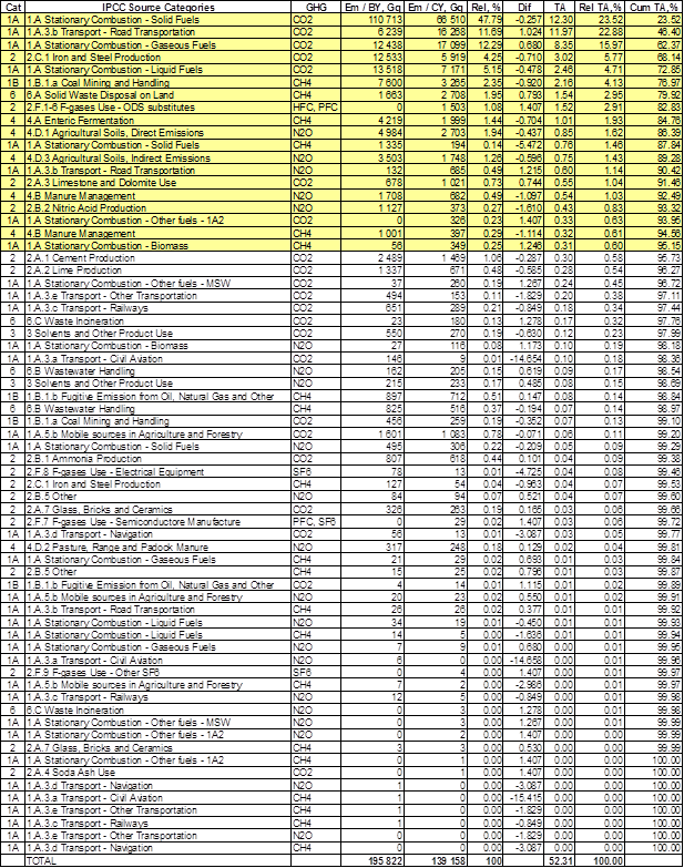
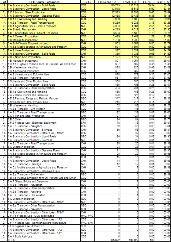
ES 2 Summary of National Emission and Removal Related Trends and Emission and Removals from KP-LULUCF Activities

ES 2.1 GHG inventory

In 2010, the most important GHG in the Czech Republic was CO₂ contributing 85.5 % to total national GHG emissions and removals expressed in CO₂eq., followed by CH₄ 7.8 % and N₂O 5.6 %. PFCs, HFCs and SF₆ contributed for 1.16 % to the overall GHG emissions in the country. CO₂ net emissions from LULUCF totalled at -4.2 % from the overall GHG emissions.

Tab. ES 2‑1 provides data on GHG emissions in comparison of overall trend from 1990 to 2010. For overview of GHG emission and removals by categories please see chapter ES 3 on page 15.

Tab. ES 2‑1 GHG emission/removal overall trends

	Base year	2010	Base year	2010	Trend
	[Gg CO₂ eq.]		[%]
CO₂ emissions	165097	119866	85.9	89.7	-27.4
[1]CO₂ (LULUCF)	-3749	-5666	-2.0	-4.2	51.1
CO₂ Total	161348	114200	83.9	85.5	-29.2
[2]CH₄	17914	10413	9.3	7.8	-41.9
²N₂O	12865	7477	6.7	5.6	-41.9
F-gases	78	1549	0.04	1.16	19.9-times
Total	192204	133639	100	100	-30.5

Over the period 1990 - 2010 CO₂emissions and removals decreased by 30.5 %, CH₄ emissions decreased by 41.9 % during the same period mainly due to lower emissions from 1 Energy, 4 Agriculture and 6 Waste; N₂O emissions decreased by 41.9 % over the same period due to emission reduction in 4 Agriculture and despite increase from the 1A3 Transport category. Emissions of HFCs and PFCs increased by orders of magnitude, whereas SF₆ emissions decreased significantly, resulting the overall F-gases trend at almost 20-times increase in CO₂eq.

ES 2.2 KP-LULUCF activities

Emission and removal estimates of GHGs for applicable KP-LULUCF activities in the years 2008, 2009 and 2010 are presented in Tab. ES 2‑2.

Tab. ES 2‑2 Summary of GHG emissions and removals for KP LULUCF activities [Gg CO₂ eq.]

Year	Article 3.3 activities		Article 3.4 activities
Year	Afforestration and Reforestration	Deforestation	Forest Management*	Cropland Management	Grazing Land Management	Revegetation
2008	-272	160	-4404	NA	NA	NA
2009	-295	170	-6441	NA	NA	NA
2010	-322	207	-5096	NA	NA	NA

*) Net emissions or removals / accounting quantity

ES 3 Overview of Source and Sink Category Emission Estimates and Trends, including KP-LULUCF Activities

ES 3.1 GHG inventory

Tab. ES 3‑1 Overview of GHG emission/removal overall trends by categories

			Base year	2010	Base year	2010	Trend
					Category share [%]		[%]
1. Energy			157048.2	115204.9	81.7	86.2	-26.6
	A. Fuel Combustion (Sectoral Approach)		148090.4	110954.0	94.3	96.3	-25.1
		1. Energy Industries	58007.9	56251.1	36.9	48.8	-3.0
		2. Manufacturing Industries and Construction	46885.4	23806.9	29.9	20.7	-49.2
		3. Transport	7766.8	17448.4	4.9	15.1	124.7
		4. Other Sectors	33802.9	12340.0	21.5	10.7	-63.5
		5. Other	1627.5	1107.7	1.0	1.0	-31.9
	B. Fugitive Emissions from Fuels		8957.7	4250.9	5.7	3.7	-52.5
		1. Solid Fuels	8056.2	3524.7	5.1	3.1	-56.2
		2. Oil and Natural Gas	901.5	726.2	0.6	0.6	-19.5
2. Industrial Processes			19602.8	12061.1	10.2	9.0	-38.5
	A. Mineral Products		4832.8	3428.4	24.7	28.4	-29.1
	B. Chemical Industry		2032.5	1110.7	10.4	9.2	-45.4
	C. Metal Production		12659.9	5973.0	64.6	49.5	-52.8
	F. Consumption of Halocarbons and SF₆[3]		76.1	1549.0	0.4	12.8	1936.6
3. Solvent and Other Product Use			764.8	502.7	0.4	0.4	-34.3
4. Agriculture			15733.2	7777.3	8.2	5.8	-50.6
	A. Enteric Fermentation		4219.4	1998.8	26.8	25.7	-52.6
	B. Manure Management		2709.6	1079.3	17.2	13.9	-60.2
	D. Agricultural Soils(3)		8804.2	4699.2	56.0	60.4	-46.6
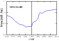
5. Land Use, Land-Use Change and Forestry[4]			-3617.9	-5518.5	-1.9	-4.1	52.5
	A. Forest Land		-4947.0	-5440.1	136.7	98.6	10.0
	B. Cropland		1336.5	138.9	-36.9	-2.5	-89.6
	C. Grassland		-127.9	-371.3	3.5	6.7	190.3
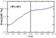
	D. Wetlands		22.5	34.2	-0.6	-0.6	52.0
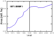
	E. Settlements		86.1	117.5	-2.4	-2.1	36.5
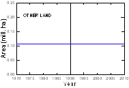
	G. Other		11.8	2.3	-0.3	0.0	-80.9
6. Waste			2673.2	3611.8	1.4	2.7	35.1
	A. Solid Waste Disposal on Land		1662.6	2708.2	62.2	75.0	62.9
	B. Waste-water Handling		987.0	720.5	36.9	19.9	-27.0
	C. Waste Incineration		23.6	183.1	0.9	5.1	676.2
*Total CO₂ Equivalent Emissions* including LULUCF			*192204.3*	*133639.4*	*100.0*	*100.0*	*-30.5*
*Total CO₂ Equivalent Emissions* excluding LULUCF			*195822.25*	*139157.86*	-	-	-

NO, NA, NE sub-categories omitted

In 2010, 115205 Gg CO₂eq., that are 86.2 % of national total emissions (including 5 Land Use, Land-Use Change and Forestry) arose from 1 Energy; 96 % of these emissions arise from fuel combustion activities. The most important sub-category of 1 Energy with 49 % of total sectoral emissions in 2010 is 1A1 Energy Industries, 1A2 Manufacturing Industries and Construction responses for 21 % and 1A3 Transport for 15 % of total sectoral emissions. From 1990 to 2010 emissions from 1 Energy decreased by 26.6 %.

2 Industrial Processes is the second largest category with 9.0 % of total GHG emissions (including 5 Land Use, Land-Use Change and Forestry) in 2010 (12061 Gg CO₂eq.); the largest sub-category is 2C Metal Production with 50% of sectoral share. From 1990 to 2010 emissions from 2 Industrial Processes decreased by 38.5 %.

In 2010, 0.4 % of total GHG emissions (including 5 Land Use, Land-Use Change and Forestry) in the Czech Republic (506 Gg CO₂eq.) arose from the category 3 Solvent and Other Product Use. From 1990 - 2010 emissions from 3 Solvent and Other Product Use decreased by 34.3 %.

4 Agriculture is the third largest category in the Czech Republic with 5.8 % share of total GHG emissions (including 5 Land Use, Land-Use Change and Forestry) in 2010 (7 777 Gg CO₂eq.); 60 % of emissions is coming from 4D Agricultural Soils. From 1990 to 2010 emissions from 4 Agriculture decreased by 50.6 %.

5 Land Use, Land-Use Change and Forestry is the only category where removals exceed emissions. Net removals from this category increased from 1990 to 2010 by 52.5 % to 5518 Gg CO₂eq.

2.7 % of the national total GHG emissions (including 5 Land Use, Land-Use Change and Forestry) in 2010 arose from 6 Waste. 75 % share of GHG emissions arose from 6C Solid waste disposal on land. Emissions from 6 Waste increased from 1990 to 2010 by 35.1 % to 3612 Gg CO₂eq.

ES 3.2 KP-LULUCF activities

Emission and removals estimates of GHGs for the KP LULUCF activities in the years 2008, 2009 and 2010 are presented in Tab. ES 3‑2.

Tab. ES 3‑2 Summary

	CO₂ emissions	CO₂ removals	CH₄	N₂O
	CO₂ emissions	CO₂ removals	CH₄	N₂O
2008	159.8	-4 834.2	6.8	0.05
2009	169.8	-6 869.6	5.8	0.04
2010	206.4	-5 559.7	6.11	0.04

ES 4 Other information

ES 4.1 Overview of Emission Estimates and Trends of Indirect GHGs and SO₂

Emission estimates of indirect GHGs and SO₂ for the period from 1990 to 2010 are presented in Tab. ES 4‑1.

Tab. ES 4‑1 Indirect GHGs and SO₂ for 1990 to 2010 [Gg]

	NO_x	CO	NMVOC	SO₂
1990	742	1 071	311	1 876
1991	732	1 157	273	1 772
1992	708	1 162	257	1 559
1993	691	1 194	233	1 469
1994	451	1 075	255	1 290
1995	430	932	215	1 095
1996	447	965	265	934
1997	471	981	272	981
1998	414	812	267	442
1999	391	726	247	269
2000	397	680	244	264
2001	333	687	220	251
2002	319	587	203	237
2003	326	630	203	232
2004	334	622	198	227
2005	279	556	182	219
2006	284	540	179	211
2007	286	584	174	217
2008	263	498	166	174
2009	253	454	151	173
2010	241	455	150	170
Trend [%]	-67.6	-57.5	-51.9	-90.9
NEC[5]	286	-	220	283

Emissions of indirect greenhouse gases decreased from the period from 1990 to 2010: for NO_x by 67.6 %, for CO by 57.5 %, for NMVOC by 51.9 % and for SO₂ by 90.9 %. The most important emission source for indirect greenhouse gases and SO₂ are fuel combustion activities.

ES 4.2 UNFCCC review related resubmission October 2012

Zaoblený obdélník: This chapter contains all the referenced changes in provisions of National Inventory Report issued by the potential problems identified during UNFCCC centralised review in September 2012

This edition is resubmitted version of National Greenhouse Gas Inventory Report of the Czech Republic. The resubmission was recommended by ERT on 9 September 2012 in Saturday paper submitted to the Czech Republic with the list of Potential Problems. Czech Republic provides in this version additional information or revised estimates of emissions corresponding to the identified Potential Problems.

The first potential problem is related to the Energy sector to the Stationary combustion. The default emission factors given in 2006 Guidelines were replaced by default emission factors given in Revised 1996 Guidelines. The revised estimates influenced all tables containing the emission estimates and emission factors in chapter 3 Energy, Specifically the tables 3-2, 3-3, 3-14 (See revised table 3-14 below) and also the chapter 3.7.1. For details please see attached Saturday paper-response.

The response to the potential problem related to the category 1.A.3.a Civil Aviation is given in attached Saturday paper-response.

The potential problem related to the emissions associated with charcoal use was solved and the description is provided in response to the Saturday paper. These emissions don’t influence final tables with emission estimates since the biomass is not included in resulting CO₂ emissions.

CH₄ emissions from charcoal production were newly estimated. In the next submission the explanation of this source of emission will be given in chapter for 1.B.1.b Coal transformation category.

IPCC GPG was applied and available information on production of crops (alfalfa and clover) and national values were used to estimate N₂O emissions in response to the potential problem related to the 4.D.1.3 N-fixing crops category. The emissions from Agricultural soils, Direct Soil Emissions, N-fixing crops (4.D.1.3) reported in the last submission 2012 will be increased by the amount of emissions calculated in terms of this recalculation. The description will be given in next submission in chapter 6.4.

N₂O Direct Soil Emissions from Crop Residue (potatoes and sugarbeet) were estimated applying the IPCC GPG and using available information on production of these crops (potential problem for category 4.D.1.4). The detailed response to this potential problem is given in Saturday paper-response. Detailed description will be given in next submission in chapter 6.4.

The response to the potential problems related to the 6.A Solid Waste Disposal and 6.C Waste Incineration given in attached Saturday paper-response.

All changes provided in response to the Saturday paper influence also the chapter 12.5 Calculation of the Commitment Period Reverse. The calculation of five times the most recent inventory (2010) is given below

5 x 139 523 382= 697 616 911 (t) CO_2eq

Revised Tab. 3-14 Net caloricic values (NCV), CO₂ emission factors and oxidation factors used in the Czech GHG inventory

Fuel (IPCC 1996 Guidelines	NCV	CO₂ EF ^a)	Oxidation	CO₂ EF ^b)
definitions)	[TJ/Gg]	[t CO₂/TJ]	factor ^e)	[t CO₂/TJ]
Crude Oil	42.40	73.33	0.99	72.60
Gas / Diesel Oil	42.75	74.07	0.99	73.33
Residual Fuel Oil	39.59	77.37	0.99	76.59
LPG	43.82	63.07	0.995	62.75
Naphtha	43.96	73.33	0.99	72.60
Bitumen	40.19	80.67	0.99	79.86
Lubricants	40.19	73.33	0.99	72.60
Petroleum Coke	37.50	100.83	0.98	98.82
Other Oil	39.82	73.33	0.99	72.60
Coking Coal ^d)	29.39	93.24	0.98	91.38
Other Bituminous Coal ^d)	23.19	93.24	0.98	91.38
Lignite (Brown Coal) ^d)	12.67	99.99	0.98	97.99
Brown Coal Briquettes	20.82	94.60	0.98	92.71
Coke Oven Coke	27.93	108.17	0.98	106.00
Coke Oven Gas (TJ/mill. m³)	15.62^c)	47.67	0.995	47.43
Natural Gas (TJ/Gg)	57.22	56.10	0.995	55.82
Natural Gas (TJ/mill. m³)	34.33^c)	56.10	0.995	55.82

a) Emission factor without oxidation factor

b) Resulting emission factor with oxidation factor

c) TJ/mill. m³, t= 15°C, p = 101.3 kPa

d) Country specific values of CO₂ EFs

e) Oxidation factors values used for national inventory of greenhouse gases are 0.995 for gaseous fuels, 0.99 for liquid fuels and 0.98 for solid fuels

Inventory related potential problems identified by ERT during centralised UNFCCC review 2012

With reference to the Guidelines for review under Article 8 of the Kyoto Protocol, the ERT requests that additional information and/or revised estimates for the 2010 greenhouse gas (GHG) inventory corresponding to the potential problems identified in this paper (see attached tables) be forwarded to the ERT, through the UNFCCC secretariat, not later than by 22 October 2012.

Should the Czech Republic decide to submit by 22 October 2012, in response to some or all potential problems, revised estimates of its GHG emissions, the ERT requests that the revised estimates contain the following:

· Relevant background information and a descriptive summary of the revisions made by the Czech Republic in its 2012 inventory submission, in particular in the year 2010 with respect to:

1. CO₂ emissions from 1.A Stationary Combustion (liquid fuels);

2. CO₂, CH₄ and N₂O emissions from 1.A.3.a Civil Aviation;

3. CH₄ and N₂O emissions from 1.A.4.b Residential;

4. CH₄ emissions from 1.B.1.b Solid Fuel Transformation;

5. N₂O emissions from 4.D.1.3 N-fixing crops;

6. N₂O emissions from 4.D.1.4 Crop residue;

7. CH₄ emissions from 6.A Solid Waste Disposal;

8. CH₄ and N₂O emissions from 6.C Waste Incineration;

· A complete resubmission of the 2012 CRF tables, reflecting the revised estimates;

· Party’s revision of the calculation of the commitment period reserve, based on the recalculated emissions reported for 2010, if the calculation of the commitment period reserve is based on the inventory and not the assigned amount.

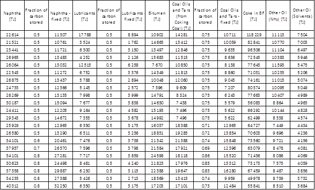
1. Stationary combustion, liquid fuels (1.A)

According to the recommendation of ERT the recalculation of CO₂ emissions from 1.A Stationary combustion were performed by using EF provided by the 1996 Revised IPCC Guidelines for the period 1995-2010. The ERT recommended recalculating only liquid fuels, but the party is convinced that it would lead to inconsistencies in reporting and therefore are used emission factors given by 1996 Revised IPCC Guidelines also for gaseous fuels and biomass. Country specific emission factors are used for Coking Coal, Other Bituminous Coal and for Brown Coal+Lignite; for the rest of solid fuels the default emission factors given by 1996 Revised IPCC Guidelines are used. Because the 2006 IPCC Guidelines emission factors were used for the period 1995-2010, the emissions in1990-1994 period remains the same before and after this recalculation. Since emission factors given by 1996 Revised IPCC Guidelines and by 2006 IPCC Guidelines not differ too much, the distinction between original estimates and corrected/recalculated estimates is not too significant.

1.A Stationary combustion

year	Original estimate (Gg CO₂)	Corrected estimate (Gg CO₂)
1990	145 893.92	145 893.92
1991	140 063.18	140 063.18
1992	124 431.60	124 431.60
1993	123 371.42	123 371.42
1994	113 653.39	113 653.39
1995	115 462.71	115 635.36
1996	119 294.50	119 461.86
1997	115 698.41	115 863.28
1998	109 440.37	109 589.65
1999	104 419.79	104 558.55
2000	113 232.44	113 376.53
2001	113 805.04	113 969.03
2002	110 521.69	110 676.04
2003	113 000.32	113 157.71
2004	114 029.53	114 175.45
2005	115 105.90	115 260.48
2006	115 807.16	115 976.74
2007	115 313.18	115 494.52
2008	110 997.99	111 193.95
2009	105 726.36	105 891.26
2010	109 181.21	109 353.56

2. Energy, Transport, Civil Aviation (1.A.3.a)

The jet kerosene data were recalculated in last submission, because there were several discrepancies and inconsistencies between years relating to the consumption of jet kerosene in civil aviation (ERT foundation). The total consumption of jet kerosene in the Czech Republic was divided into five categories (Civil Aviation, Aviation Bunkers, Army, Industry and Commercial/Institutional). The jet kerosene consumption as well as relevant emissions from categories Army, Industry, Commercial/Institutional is not reported in CRF Reporter in Transport sector 1A3 (or International Bunkers 1C1), but in sectors 1A5bi, 1A2f and 1A4a. Other two categories (Civil Aviation 1A3a and Aviation Bunkers 1C1a) were divided based on expert judgement in the whole time period. The main criteria were passengers transport (now there is only one regular domestic line between airports Praha and Ostrava) and transport of goods. The regular domestic flights (36 TJ) using jet kerosene in comparison with international flights (13 387 TJ) are represented in the Czech Republic by a very small percentage. In IEA data (1 161 TJ) jet kerosene consumption from categories Army, Industry, Commercial/Institutional is included in the category Civil Aviation so it is not used for aviation or for transport at all. More detailed description is given in the NIR 2012 on the page 114 (chapter 3.7.3 1A3 Mobile Combustion - Source-specific recalculations). The following table shows the distribution of jet kerosene consumption in CRF tables in comparison with IEA data. It is obvious that the total sum of jet kerosene is the same in both cases.

Distribution of jet kerosene consumption in CRF Reporter and IEA data.

CRF Reporter
		[kt]	[TJ]
Total		330.00	14 289
Civil Aviation	1A3a	0.83	35.9
Aviation Bunkers	1C1a	309.17	13 387.0
Army	1A5bi	15.00	649.5
Industry	1A2f	2.00	86.6
Commercial/Institutional	1A4a	3.00	129.9
IEA data
		[kt]	[TJ]
Total		330.00	14 289
Domestic Aviation		27.00	1 169.1
International Aviation		303.00	13 120.0

3. Energy, Other Sectors, Residential (1.A.4.b)

According to the recommendation of ERT the calculation of CH₄ and N₂O emissions associated with charcoal use in category 1.A.4.b Residential were performed by using EF provided by the 1996 Revised IPCC Guidelines (Table 1-7- in Volume 3 for CH₄, Table 1-8 in Volume 3 for N₂O). With respect to available data about imports and exports was calculated apparent consumption of charcoal which was then used as activity data. Final emissions from charcoal use were then included in emissions from biomass in 1.A4.b category. Please see the table for the results.

1.A.4.b Residential - Biomass

	Original estimate	New estimate	Original estimate	New estimate
	(Gg CH₄)		(Gg N₂O)
1990	1.76	1.78	0.02	0.02
1991	1.73	1.74	0.02	0.02
1992	1.76	1.77	0.02	0.02
1993	1.50	1.51	0.02	0.02
1994	1.51	1.51	0.02	0.02
1995	7.20	7.20	0.10	0.10
1996	7.55	7.56	0.10	0.10
1997	7.46	7.46	0.10	0.10
1998	8.49	8.49	0.11	0.11
1999	8.64	8.66	0.12	0.12
2000	9.13	9.14	0.12	0.12
2001	10.06	10.07	0.13	0.13
2002	8.85	8.87	0.12	0.12
2003	10.35	10.38	0.14	0.14
2004	11.03	11.06	0.15	0.15
2005	11.12	11.17	0.15	0.15
2006	12.04	12.09	0.16	0.16
2007	13.98	14.04	0.19	0.19
2008	13.25	13.31	0.18	0.18
2009	13.05	13.11	0.17	0.17
2010	14.55	14.62	0.19	0.19

4. Energy, Fugitive Emissions from Solid Fuels, Solid Fuel Transformation (1.B.1.b)

According to the recommendation of ERT the calculation of CH₄ emissions from charcoal production were performed by using EF provided by the 1996 Revised IPCC Guidelines (Table 1-14); the value of 1000 kg/TJ of charcoal produced were used. Since there are no available official activity data about charcoal production in the Czech Republic the un-official data from FAOSTAT statistics were used. The missing data were extrapolated. The default net calorific value 30 MJ/kg (Table 1-13 in 1996 Revised IPCC Guidelines) was used to convert activity data to the energy units. Resulting CH₄ emissions please see in the table.

1.B.1.b Solid Fuel Transfromation

	Production	Production	CH₄ emissions
	Gg/year	TJ/year	Gg/year
1990	1.00	30.00	0.03
1991	1.00	30.00	0.03
1992	1.00	30.00	0.03
1993	1.00	30.00	0.03
1994	1.00	30.00	0.03
1995	1.00	30.00	0.03
1996	1.00	30.00	0.03
1997	1.00	30.00	0.03
1998	1.80	54.00	0.05
1999	2.60	78.00	0.08
2000	3.40	102.00	0.10
2001	4.20	126.00	0.13
2002	5.00	150.00	0.15
2003	6.00	180.00	0.18
2004	6.00	180.00	0.18
2005	6.00	180.00	0.18
2006	6.00	180.00	0.18
2007	6.00	180.00	0.18
2008	6.00	180.00	0.18
2009	6.00	180.00	0.18
2010	6.60	198.00	0.20

5. Agriculture, Agricultural soils, Direct Soil Emissions, N-fixing crops (4.D.1.3)

IPCC GPG was applied and available information on production of crops (alfalfa and clover) and national values were used to estimate N₂O emissions. The information of production comes from Czech Statistical Office (CSO). The country-specific data of the fraction of nitrogen (Frac_NCRBF); and the fraction of dry matter content (Frac_DM) in aboveground biomass of forage crops were applied to the emission inventory. For the fraction of dry matter and fraction of nitrogen, the materials (results of research projects) of Faculty of Agronomy, South Bohemia University, were used.

Production data (tonnes)

	Clover	Alfalfa
1990	1 344 264	1 087 610
1991	1 647 742	1 522 470
1992	1 311 256	1 278 921
1993	1 256 243	1 213 911
1994	1 068 677	1 203 048
1995	1 070 732	1 123 483
1996	982 389	1 036 611
1997	946 568	883 871
1998	708 666	742 565
1999	676 221	725 922
2000	697 727	755 398
2001	669 056	760 707
2002	504 406	661 588
2003	375 074	500 186
2004	485 900	672 700
2005	458 844	695 097
2006	433 989	667 758
2007	432 315	610 479
2008	386 358	583 724
2009	376 877	587 221
2010	337 526	527 413

	Frac_DM*	Frac_NCRBF*	EF₁**
Clover	0.15	0.19	0.0125
Alfalfa	0.18	0.21	0.0125

*data www.zf.jcu.cz, Jeteloviny - study material of JCU

** default IPCC 2000, Table 4-17, page 4.60

These equations were used to estimate direct N₂O emissions from Agricultural soils - N-fixing crops:

FBN = Crop * FracDM * FracNCRBF

N₂O Emissions = FBN * EF1*44/28

The N₂O Direct Soil Emissions from N-fixing crops (clover and alfalfa production) are presented in the following table.

	N input (t N)		Emissions N₂O (Gg)			Emissions CO₂ eq. (Gg)
	Clover	Alfalfa	Clover	Alfalfa	Total	Clover	Alfalfa	Total
1990	38 312	41 112	0.753	0.808	1.560	233.3	250.3	483.6
1991	46 961	57 549	0.922	1.130	2.053	286.0	350.4	636.4
1992	37 371	48 343	0.734	0.950	1.684	227.6	294.4	521.9
1993	35 803	45 886	0.703	0.901	1.605	218.0	279.4	497.4
1994	30 457	45 475	0.598	0.893	1.492	185.5	276.9	462.4
1995	30 516	42 468	0.599	0.834	1.434	185.8	258.6	444.4
1996	27 998	39 184	0.550	0.770	1.320	170.5	238.6	409.1
1997	26 977	33 410	0.530	0.656	1.186	164.3	203.4	367.7
1998	20 197	28 069	0.397	0.551	0.948	123.0	170.9	293.9
1999	19 272	27 440	0.379	0.539	0.918	117.4	167.1	284.4
2000	19 885	28 554	0.391	0.561	0.951	121.1	173.9	295.0
2001	19 068	28 755	0.375	0.565	0.939	116.1	175.1	291.2
2002	14 376	25 008	0.282	0.491	0.774	87.5	152.3	239.8
2003	10 690	18 907	0.210	0.371	0.581	65.1	115.1	180.2
2004	13 848	25 428	0.272	0.499	0.771	84.3	154.8	239.2
2005	13 077	26 275	0.257	0.516	0.773	79.6	160.0	239.6
2006	12 369	25 241	0.243	0.496	0.739	75.3	153.7	229.0
2007	12 321	23 076	0.242	0.453	0.695	75.0	140.5	215.5
2008	11 011	22 065	0.216	0.433	0.650	67.1	134.4	201.4
2009	10 741	22 197	0.211	0.436	0.647	65.4	135.2	200.6
2010	9 619	19 936	0.189	0.392	0.581	58.6	121.4	180.0

The emissions from Agricultural soils, Direct Soil Emissions, N-fixing crops (4.D.1.3) reported in the last submission 2012 will be increased by the amount of emissions calculated in terms of this recalculation as shown in the last table column.

The recalculations required by ERT in 4.D.1.3 category will cause an increase of Direct emissions from agricultural soils of 6.6 %.

6. Agriculture, Agricultural soils; Direct Soil Emissions, Crop Residue (4.D.1.4)

N₂O Direct Soil Emissions from Crop Residue (potatoes and sugarbeet) were estimated applying the IPCC GPG and using available information on production of these crops. The source of information about crop production is Czech Statistical Office (CSO). The default N₂O EFs and default values for other relevant parameters were used in accordance with the IPCC GPG methodology.

The equation 4.29 (Tier 1b, GPG IPCC 2000, page 4.59) of the IPCC GPG was used to estimate these emissions. The default N₂O emission factor for both crops (Table 4-17, IPCC 2000 GPG, page 4.60), the default values for the fractions of nitrogen in potatoes and sugarbeet (Table 4-16, IPCC 2000, page 4.58) and default fraction of crop residue that is removed from the field as crop (Table 4-17, IPCC 1996, Reference Manual, page 4.85) were used. The country- specific data for dry matter fraction was used: The value of FracDM for potatoes is based on study Cabajova, MU LF Brno (2009) and corresponds to other available sources. The value of FracDM for sugarbeet is based on study Blaha, CZU Praha (1986) and corresponds to other available sources. Both national parameters belong to interval of IPCC default values. The fraction of crop residue that is burned on the field equals zero.

Production data (tonnes)

	Potatoes	Sugarbeet
1990	1 755 000	4 026 000
1991	2 043 205	4 008 693
1992	1 969 233	3 871 498
1993	2 395 810	4 308 286
1994	1 231 035	3 240 124
1995	1 330 119	3 711 602
1996	1 800 272	4 315 566
1997	1 401 663	3 721 980
1998	1 519 768	3 479 426
1999	1 406 832	2 690 948
2000	1 475 992	2 808 839
2001	1 130 477	3 529 005
2002	900 843	3 832 466
2003	682 511	3 495 148
2004	861 798	3 579 280
2005	1 013 000	3 495 611
2006	692 189	3 138 300
2007	820 536	2 889 900
2008	769 561	2 884 645
2009	752 539	3 038 220
2010	665 176	3 064 986

	Frac_NCRO	Res/Crop	Frac_DM	EF₁
Potatoes	0.011	0.40	0.30	0.0125
Sugarbeet	0.004	0.20	0.12	0.0125

These equations were used to estimate direct N₂O emissions from Agricultural soils – Crop Residue:

F_CR = Crop * Res/Crop * Frac_DM * Frac_NCRO*1 (Frac_burn, Frac_fuel etc. equal zero)

Emissions = F_CR * EF₁*44/28

	N input (t N)		Emissions N₂O (Gg)			Emissions CO₂ eq. (Gg)
	Potatoes	Sugarbeet	Potatoes	Sugarbeet	Total	Potatoes	Sugarbeet	Total
1990	2317	386	0.046	0.008	0.053	14.1	2.4	16.5
1991	2697	385	0.053	0.008	0.061	16.4	2.3	18.8
1992	2599	372	0.051	0.007	0.058	15.8	2.3	18.1
1993	3162	414	0.062	0.008	0.070	19.3	2.5	21.8
1994	1625	311	0.032	0.006	0.038	9.9	1.9	11.8
1995	1756	356	0.034	0.007	0.041	10.7	2.2	12.9
1996	2376	414	0.047	0.008	0.055	14.5	2.5	17.0
1997	1850	357	0.036	0.007	0.043	11.3	2.2	13.4
1998	2006	334	0.039	0.007	0.046	12.2	2.0	14.2
1999	1857	258	0.036	0.005	0.042	11.3	1.6	12.9
2000	1948	270	0.038	0.005	0.044	11.9	1.6	13.5
2001	1492	339	0.029	0.007	0.036	9.1	2.1	11.1
2002	1189	368	0.023	0.007	0.031	7.2	2.2	9.5
2003	901	336	0.018	0.007	0.024	5.5	2.0	7.5
2004	1138	344	0.022	0.007	0.029	6.9	2.1	9.0
2005	1337	336	0.026	0.007	0.033	8.1	2.0	10.2
2006	914	301	0.018	0.006	0.024	5.6	1.8	7.4
2007	1083	277	0.021	0.005	0.027	6.6	1.7	8.3
2008	1016	277	0.020	0.005	0.025	6.2	1.7	7.9
2009	993	292	0.020	0.006	0.025	6.0	1.8	7.8
2010	878	294	0.017	0.006	0.023	5.3	1.8	7.1

The emissions from Agricultural soils, Direct Soil Emissions, Direct Soil Emissions, Crop Residue (4.D.1.4) reported in the last submission 2012, will be increased by the amount of emissions calculated in terms of this recalculation as shown in the last table column.

The recalculations required by ERT in 4.D.1.4 category will cause an increase of total Direct emissions from agricultural soils of 0.3 %.

Detailed Agriculture recalculation comparison

	OLD_Subm. 2012		NEW_recalculated		4D.1 - Direct emissions from AS
	4D.1.3	4D.1.4	4D.1.3	4D.1.4	OLD	NEW	INC (%)
1990	0.182	3.000	1.742	3.053	16.077	17.690	10.0
1991	0.237	2.672	2.290	2.733	13.420	15.534	15.8
1992	0.244	2.262	1.928	2.320	11.349	13.091	15.3
1993	0.269	2.244	1.874	2.314	10.081	11.756	16.6
1994	0.193	2.303	1.685	2.341	9.932	11.462	15.4
1995	0.171	2.233	1.605	2.274	10.069	11.544	14.6
1996	0.160	2.242	1.480	2.297	9.404	10.779	14.6
1997	0.123	2.331	1.309	2.374	9.604	10.833	12.8
1998	0.157	2.248	1.105	2.294	9.385	10.379	10.6
1999	0.142	2.323	1.060	2.365	9.414	10.374	10.2
2000	0.103	2.148	1.054	2.192	9.256	10.251	10.7
2001	0.113	2.440	1.052	2.476	9.714	10.689	10.0
2002	0.084	2.241	0.858	2.272	9.465	10.270	8.5
2003	0.087	1.916	0.668	1.940	8.439	9.044	7.2
2004	0.119	2.912	0.890	2.941	9.775	10.575	8.2
2005	0.135	2.557	0.908	2.590	9.142	9.948	8.8
2006	0.124	2.138	0.863	2.162	8.828	9.591	8.6
2007	0.093	2.369	0.788	2.396	9.178	9.900	7.9
2008	0.068	2.750	0.718	2.775	9.705	10.380	7.0
2009	0.089	2.587	0.736	2.612	9.090	9.762	7.4
2010	0.088	2.277	0.669	2.300	8.719	9.323	6.9

The total emissions in 4D.1 category (Direct emissions from agricultural soils) increased after recalculation by 6.9 % in 2010 (the last column in the previous table).

7. Waste, Solid waste disposal (6.A)

Amount of sludge produced in the country is estimated by using tier 1 method on the basis of population statistics. Basis for sludge production from industrial waste water treatment is industry production statistics. Wastewater treatment is split between sludge and water streams. Both of these organic pollution streams are treated by mixture of aerobic and anaerobic technologies which are accounted for in 6B – Wastewater handling using tier 1 method.

Landfilling of raw sludge is NOT occurring in the country and as such is prohibited by legislation. In actual fact ordinary MSW landfills are not even capable to accept raw sludge as they have no technical equipment to do so and direct application of sludge might damage landfill equipment (LFG capturing system, compactors etc.). In addition every wastewater treatment plant must have a sludge treatment facility (sludge digestion). Landfills DO accept product from sludge digestion - sludge that already passed process of methanisation.

Emissions from landfilling of digested sludge are accounted for under 6A – Solid waste disposal on land as a fraction of the whole landfilling emissions. GHG emissions from landfilling are based on bottom-up data (waste actually delivered at landfilling sites by its mass) and overall DOC (Degradable Organic Content) which has been determined in number of case studies.

To prevent confusion: The fact that sludge does NOT figure in landfils disposed waste composition (see NIR p.236) does NOT mean it is not accounted for in DOC calculation. It is simply below the methodology resolution – Overall landfilled mass reached 3185 kt/year compared to aprox. 6 kt/year of landfilled digested sludge (based on the table above).

Based on the facts above:

Czech republic party deems accounting of GHG emissions from wastewater sludge in accord with IPCC methodology and the current emission estimate to be accurate to the extent possible.

Summary:

• Emissions from sludge treatment (digestion) are already estimated in 6B - Wastewater handling using tier1 method.

• Table in question displays landfilled digested sludge (i.e. sludge after treatment)

• Emissions from landfilled sludge are correctly accounted for in 6A – Solid waste disposal on land using tier2 (FOD) method.

8. Waste, Waste incineration (6.C)

For the purposes of national GHG inventories NIS team relies on CENIA-CEHO statistics due to its obvious advantage in comparability/usability and transparency over the others. In other words CENIA-CEHO statistics (system ISOH) are based on bottom-up accounting. Data obtained through CZSO (e.g. the table that was most unfortunately provided to ERT) have very uncertain origin and validity (considering waste statistics). During review week Czech republic party erroneously claimed that sludge incineration is not occurring in the country. It was a misunderstanding on our part. Nonetheless sludge incineration occurs in the country and it is already accounted for in national GHG inventory.

Sludge is a very numerous family of wastes (filtration cakes, flocculants remains, industrial processes sludge etc.) and indeed some of them are incinerated. However there is not such detailed classification of waste incinerated – as recognized by waste incineration there are only two categories – “Hazardous” and “Other” (which is basically MSW). As for incinerating facilities, there are accordingly 2 types - those which can incinerate MSW and those which can incinerate hazardous waste (toxic, clinical, industrial). Because of its instability (hygienically and chemically) sludge can only be incinerated in facilities for hazardous waste. Having access to bottom-up data from all waste incineration facilities NIS team chose approach working with these two broad categories using aggregated facility-level data. This is fairly accurate approach because incinerators do have certified weights (they claim fees for mass incinerated) and every incinerated ton of waste gets into the accounting system. Unfortunately there is no source of information on incinerated waste composition so only emission estimation aproach based on general aggregated emission factor could be used. Important fact is that the incinerated sludge mass (however uncertain) is already present in currently used activity data. Currently used approach slightly over-estimates the emissions this fact is demonstrated in attached spreadsheet where a reference calculation based on data from CZSO (table 3-29) have been conducted. CH₄ EF used is from IPCC 2006 Guidelines (as it is not present in IPCC 1996 Guidelines or GPG), N₂O and CO₂ EFs are from GPG. If emission estimate is conducted with the suggested methodology the result is lower aggregated emissions by 1.74% in 2010 (category 6C). This is caused by default EF for sludge being slightly higher for N₂O and CH₄ but considerably lower for fossil CO₂. Czech republic party does not desire to use this method to lower its GHG emissions due to unreliability of incinerated sludge data source, which could only lead to higher overall uncertainty.

Based on the facts above:

Czech republic party deems accounting of GHG emissions from sludge incineration in accord with IPCC methodology and the current emission estimate to be accurate to the extent possible.

Summary:

• Emissions from sludge incineration are already reported in 6C as unspecified compound of emissions from hazardous waste incineration.

• Use of aggregated default emission factor does NOT lead to underestimation of emissions from this waste stream. As a matter of fact the emissions are slightly overestimated, pursuing the safety precautions of GHG inventory NOT being underestimated.

Part 1: Annual inventory submission

1 Introduction and general issues

1.1 Background information

1.1.1 Climate change

Greenhouse gases (i.e. gases that contribute to the greenhouse effect) have always been present in the atmosphere, but now the concentrations of a number of them are increasing as a result of human activity. Over the past century, the atmospheric concentrations of carbon dioxide (CO₂), methane (CH₄), nitrous oxide (N₂O) and halogenated hydrocarbons, i.e. greenhouse gases, have increased as a consequence of human activity. Greenhouse gases prevent the radiation of heat back into space and cause warming of the climate. According to the Fourth Assessment Report of the Intergovernmental Panel on Climate Change (IPCC, 2007), the atmospheric concentrations of CO₂ have increased by 35 %, CH₄ concentrations have more than doubled and N₂O concentrations have risen by 18 %, compared with the pre-industrial era. Ground-level ozone also contributes to the greenhouse effect. The amount of ozone formed in the lower atmosphere has increased as a result of emissions of nitrogen oxides, hydrocarbons and carbon monoxide.

Relatively new, man-made greenhouse gases that are entering the atmosphere cause further intensification of the greenhouse effect. These include, in particular, a number of substances containing fluorine (F-gases), among them HFCs (hydrofluorocarbons). HFCs are used instead of ozone-layer-depleting CFCs (freons) in refrigerators and other applications, and their use is on the increase. Compared with carbon dioxide, all the other greenhouse gases occur at low (CH₄, N₂O) or very low concentrations (F-gases). On the other hand, these substances are more effective (per molecule) as greenhouse gases than carbon dioxide, which is the main greenhouse gas.

The threat of climate change is considered to be one of the most serious environmental problems faced by humankind. The average surface temperature of the earth has risen by about 0.6–0.9 °C in the past 100 years and, according to the IPCC 4AR, will rise by another 1.8–4.0 °C in the next 100 years, depending on the emission scenario. The increase of the average surface temperature of the Earth, together with the increase in the surface temperature of the oceans and the continents, will lead to changes in the hydrologic cycle and to significant changes in the atmospheric circulation, which drives rainfall, wind and temperature on a regional scale. This will increase the risk of extreme weather events, such as hurricanes, typhoons, tornadoes, severe storms, droughts and floods.

In consequence of scientific indications that human activities influence the climate and an increasing public awareness about local and global environmental issues during the middle of the 1980s, climate change became part of the political agenda. The Intergovernmental Panel on Climate Change (IPCC) was established in 1988 and, two years later, it concluded that anthropogenic climate change is a global threat and asked for an international agreement to deal with the problem. The United Nations started negotiations to create a UN Framework Convention on Climate Change (UNFCCC), which came into force in 1994. The long-term goal consisted in stabilizing the amount of greenhouse gases in the atmosphere at a level where harmful anthropogenic climate changes are prevented. Since UNFCCC came into force, the Framework Convention has evolved and a Conference of the Parties (COP) is held every year. The most important addition to the Convention was negotiated in 1997 in Kyoto, Japan. The Kyoto Protocol established binding obligations for the Annex I countries (including all EU member states and other industrialized countries). Altogether, the emissions of greenhouse gases by these countries should be at least 5 % lower during 2008-2012 compared to the base year of 1990 (for fluorinated greenhouse gases, 1995 can be used as a base year). In 2001 the Czech Republic ratified the Kyoto Protocol and it came into force on February 16, 2005, even though it has not been ratified by the United States.

Under the Kyoto Protocol, the Czech Republic is committed to decrease its emissions of greenhouse gases in the first commitment period, i.e. from 2008 to 2012, by 8 % compared to the base year of 1990 (the base year for F-gases is 1995).

1.1.2 Greenhouse gas inventories

Annual monitoring of greenhouse gas emissions and removals is one of the obligations following from the UN Framework Convention on Climate Change and its Kyoto Protocol. In addition, as a result of membership in the European Union, the Czech Republic must also fulfill its reporting requirements concerning GHG emissions and removals following from Decision of the European Parliament and Council No. 280/2004/EC. This Decision also requires establishing a National Inventory System (NIS) pursuant to the Kyoto Protocol (Art. 5.1) from December 2005.

The Czech Hydrometeorological Institute (CHMI) was appointed in 1995 by the Ministry of Environment (MoE), which is the founder and supervisor of CHMI, to be the institution responsible for compiling GHG inventories. Thereafter, CHMI has been the official provider of Czech greenhouse gas emission data. The role of CHMI was improved following implementation of NIS in 2005, when CHMI was designated by MoE as the coordinating institution of the official national GHG inventory.

The inventory covers anthropogenic emissions of direct greenhouse gases CO₂, CH₄, N₂O, HFC, PFC, SF₆ and indirect greenhouse gases NO_x, CO, NMVOC and SO₂. Indirect means that they do not contribute directly to the greenhouse effect, but that their presence in the atmosphere may influence the climate in various ways. As mentioned above, ozone (O₃) is also a greenhouse gas that is formed by the chemical reactions of its precursors: nitrogen oxides, hydrocarbons and/or carbon monoxide.

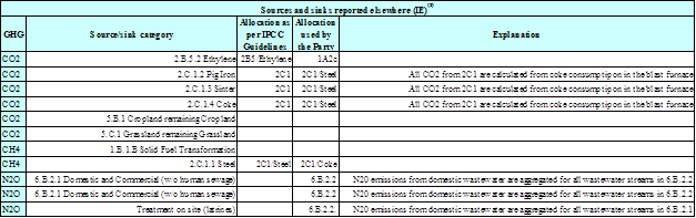
The obligations of the Kyoto Protocol have led to an increased need for international supervision of the emissions reported by the parties. The Kyoto Protocol therefore contains rules for how emissions should be estimated, reported and reviewed. Emissions of the direct greenhouse gases CO₂, N₂O, CH₄, HFCs, PFCs and SF₆ are calculated as CO₂ equivalents and added together to produce a total. Together with the direct greenhouse gases, also the emissions of NO_x, CO, NMVOC and SO₂ are reported to UNFCCC. These gases are not included in the obligations of the Kyoto Protocol. The emission estimates and removals are reported by gas and by source category and refer to 2010. Full time series of emissions and removals from 1990 to 2010 are included in the submission.

Inventories of emissions and removals of greenhouse gases were prepared according to the IPCC methodology: Revised 1996 IPCC Guidelines (IPCC, 1997); Good Practice Guidance (IPCC, 2000); Good Practice Guidance for LULUCF (IPCC, 2003); application of this general methodology under country-specific circumstances will be described in the sector-specific chapters. When a method used to estimate emissions is improved or when some gaps are identified, a need to recalculate the whole time series may arise in order to maintain consistency. This means that data presented this year can change in the next submission.

At the beginning of 2009, the Secretariat published a methodical handbook entitled “Annotated outline of the National Inventory Report including elements under the Kyoto Protocol” (UNFCCC, 2009), providing instructions on how to combine the existing requirements on reporting pursuant to decision 18/CP.8 and 14/CP.11, see (UNFCCC, 2006) with the requirements on reporting pursuant to Article 7.1 of the Kyoto Protocol given in Decision 15/CMP.1. This report attempts to follow this methodical handbook.

The current data submission (2012) for UNFCCC and for the European Community contains all the data sets for 1990 - 2010 in the form of the official UNFCCC software called CRF Reporter (version 3.4).

1.2 National Inventory System and Institutional Arrangement

The National Inventory System (NIS), as required by the Kyoto Protocol (Article 5.1) and by Decision No. 280/2004/EC, has been in place since 2005. As approved by the Ministry of Environment (MoE), which is the single national entity with overall responsibility for the national greenhouse gas inventory, the founder of CHMI and its superior institution, the established institutional arrangement is as follows:

The Czech Hydrometeorological Institute (CHMI), under the supervision of the Ministry of the Environment, is designated as the coordinating and managing organization responsible for the compilation of the national GHG inventory and reporting its results. The main tasks of CHMI consist in inventory management, general and cross-cutting issues, QA/QC, communication with the relevant UNFCCC and EU bodies, etc. Mr. Ondrej Minovsky is the representative of CHMI for NIS performance.

Sectoral inventories are prepared by sector experts from sector-solving institutions, which are coordinated and controlled by CHMI. The responsibilities for GHG inventory compilation from the individual sectors are allocated in the following way:

§ KONEKO MARKETING Ltd. (KONEKO), Prague, is responsible for compilation of the inventory in sector 1, Energy, for stationary sources including fugitive emissions

§ Transport Research Centre (CDV), Brno, is responsible for compilation of the inventory in sector 1, Energy, for mobile sources

§ Czech Hydrometeorological Institute (CHMI), Prague, is responsible for compilation of the inventory in sectors 2 and 3, Industrial Processes and Product (Solvent) Use

§ Institute of Forest Ecosystem Research Ltd. (IFER), Jilové u Prahy, is responsible for compilation of the inventory in sectors 4 and 5, Agriculture and Land Use, Land Use Change and Forestry

§ Charles University Environment Centre (CUEC), Prague, is responsible for compilation of the inventory in sector 6, Waste.

Official submission of the national GHG Inventory is prepared by CHMI and approved by the Ministry of Environment. Moreover, the MoE secures contacts with other relevant governmental bodies, such as the Czech Statistical Office, the Ministry of Industry and Trade and the Ministry of Agriculture. In addition, the MoE provides financial resources for the NIS performance to the CHMI, which annually concludes contracts with sector-solving institutions.

More detailed information about NIS is given in the Initial Report (MoE, 2006) and in the 5^th National Communication (MoE, 2009).

1.3 Inventory Preparation

1.3.1 Brief Description of the inventory process

UNFCCC, the Kyoto Protocol and the EU greenhouse gas monitoring mechanism require the Czech Republic to annually submit a National Inventory Report (NIR) and Common Reporting Format (CRF) tables. The annual submission contains emission estimates for the second but last year, so the 2012 submission contains estimates for the calendar year of 2010. The organisation of the preparation and reporting of the Czech greenhouse gas inventory and the duties of its institutions are detailed in the previous section (1.2).

The preparation of the inventory includes the following three stages:

1) inventory planning,

2) inventory preparation and

3) inventory management.

During the first stage, specific responsibilities are defined and allocated: as mentioned before, CHMI coordinates the national GHG inventory, including the planning period. Within the inventory system, specific responsibilities, “sector-solving institutions”, are defined for the different source categories, as well as for all activities related to the preparation of the inventory, including QA/QC, data management and reporting.

During the second stage, the inventory preparation process, experts from sector-solving institutions collect activity data, emission factors and all the relevant information needed for final estimation of emissions. They also have specific responsibilities regarding the choice of methods, data processing and archiving. As part of the inventory plan, the NIS coordinator approves the methodological choice. Sector-solving institutions are also responsible for performing Quality Control (QC) activities that are incorporated in the QA/QC plan, (see Chapter 1.5). All data collected, together with emission estimates, are archived (see below) and documented for future reconstruction of the inventory.

In addition to the actual emission data, the background tables of the CRF are filled in by the sector experts, and finally QA/QC procedures, as defined in the QA/QC plan, are performed before the data are submitted to the UNFCCC.

For the inventory management, reliable data management to fulfil the data collecting and reporting requirements is necessary. As mentioned above, data are collected by the experts from the sector solving institutions and the reporting requirements increase rapidly and may change over time. The data and calculation spreadsheets are stored in a central network server at CHMI, which is regularly backed up to ensure data security. The inventory management includes a control system for all documents and data, for records and their archives, as well as documentation on QA/QC activities (see Chapter 1.5).

1.3.2 Activity Data Collection

Collection of activity data is based mainly on the official documents of the Czech Statistical Office (CzSO), which are published annually, where the Czech Statistical Yearbook is the most representative example. However for industrial processes, because of the Czech Act on Statistics, production data are not generally available when there are fewer than 4 enterprises in the whole country. In such cases, inventory compilers have to rely either on specific statistical materials edited by sectoral associations or, in some cases, inventory experts have to carry out the relevant inquiries. In a few cases, the Czech register of individual sources and emissions, called REZZO, is utilized as source of activity data.

Emission estimates from Sector 1A Fuel Combustion Activities are based on the official Czech Energy Balance, compiled by the Czech Statistical Office. Data from the Czech Energy balance are processed both in the Reference Approach (TPES - primary sources data are used) and in the Sectoral Approach (data for fuel transformations and final consumptions). However, in the latter case, some additional data are required (e.g. data on transportation statistics).

So far, data from the emission trading system has been used to only a limited degree in the Czech national greenhouse gas inventory (e.g. in the sector of Industrial processes - mineral products). It was recommended to the Czech inventory team during the recent “in-country review” that the data from EU ETS be used to a greater degree. For this purpose, the team began to prepare an “improvement plan” to provide for gradual inclusion of the relevant EU ETS data in the national inventory. The next part of this “improvement plan” will consist in gradual introduction of higher tiers into the national inventory. At the present time, CHMI, in cooperation with MoE, is preparing a database of activities and emission data from the EU ETS system, which could be used in preparation of the national inventory. Consequently, it can be expected that these data will be employed more extensively only in future inventories.

1.3.3 Data Processing and Storage

Data Sector 1A Fuel Combustion Activities are processed by the system of interconnected spreadsheets, compiled in MS Excel following “Worksheets” presented in IPCC Guidelines, Vol. 2. Workbook. The system is extended by incorporating sheets with modified energy balance: these sheets represent an input data system. This system was recently a bit modified to be more transparent.

Also, in the majority of other sectors, data are processed in a similar way - by using a system of joined spreadsheets taken from the Workbook and slightly modified in order to respect national circumstances. The following examples of such cases of processing can be mentioned: agriculture, waste, fugitive emissions. On the other hand, in some cases, e.g. for solvent use, such a system is not as efficient and thus it is substituted by spreadsheets inspired by the CORINAIR methodology. For LULUCF, a specific spreadsheet system is used, respecting the national methodology.

Originally, the calculation spreadsheets related to the individual sectors were stored only in the relevant sector-solving institutions. On the basis of recommendations from the “in-country review” in 2007, a quite simple system was developed for central archiving, based on storage of documents from institutions participating in the national system in electronic form in a central folder-structured FTP data box located at CHMI. During the subsequent “in-country review” in 2009, this system was evaluated as only partly satisfactory and consequently it was decided to further improve the archiving system using more sophisticated arrangements. Due to financial limitations and employment difficulties, development of the new archiving system has been delayed. However, during the improvement plan generation period in 2011 a new archiving scheme emerged. Full implementation is planned after April 2012 (the end of submission period).

1.3.3.1 New archiving process scheme

The NIS coordinator is responsible for the administration and functioning of the archive. The archiving system is administered in accordance with the provisions of the Kyoto Protocol and the IPPC methodical recommendations.

Material archived by the sector-solving organizations

• Input data in unmodified form

• Files for transformation of original data to calculation sheets (if used)

• Calculation sheets

• Outputs from CRF

• Outputs from QA/QC

• Other relevant documents

Material archived by the coordinator

• All administrative agenda with text outputs (contracts, orders, invoices)

• Important correspondence related to the operation and functioning of NIS

• Outputs from QA/QC

• Other relevant documents

Structural arrangements of the NIS Archive

The archiving system contains and connects 4 individual units.

1) The archive of the sector-solving organization

• Functionality and administration are based on contracts with the sector-solving organizations

• Administration is provided by the sectoral organizations

2) Central storage site for sharing material in the context of NIS

• Storage site accessible at ftp://ftp.chmi.cz

• Administered by the NIS coordinator

• Contains working materials for current submissions intended for archiving

3) Central closed archive of the NIS Coordinator

• Internal central archive, administered by the NIS coordinator

• Contains all the officially archived materials

• The content of the archive is stored in duplicate on special media designed for data archiving

• The archive is located in the seat of the coordinator (CHMI – Prague Komořany)

• Entries in the archive are always performed as of 30 June of the relevant year of submission and a detailed records of them is also archived.

• Entries in the archive are also performed after the end of re-submissions or during any other unplanned intervention into the database or text part of already archived submissions.

• Prior to archiving, data for archiving must be checked and authorized by the QA/QC guarantor of the relevant sectoral organization.

4) Central accessible archive

• Mirror image of the central closed archive, available on the internet

• Does not contain sensitive documents, but does contain a complete list of archived files

• Available at portal.chmi.cz

• Administered by the NIS coordinator

• Up-dating corresponds to the entries in the Central closed archive, available a maximum of 3 working days after completion of archiving.

1.4 Brief General Description of Methodology

The methods used in the Czech greenhouse gas inventory are consistent with the IPCC methodology, which has been prepared for the purpose of compilation of national inventories of anthropogenic GHG emissions and removals. The existing and valid version of the IPCC methodology consists of the Revised 1996 IPCC Guidelines (IPCC 1997), IPCC Good Practice Guidance (IPCC 2000), IPCC Good Practice Guidance for LULUCF (IPCC 2003) and, in well-founded cases (respecting national circumstances), also 2006 IPCC Guidelines for National Greenhouse Gas Inventories (IPCC 2006).

Depending on the complexity of the calculation and types of emission factors used (generally recommended - default, country-specific, site-specific and technology-specific), the approaches described in the IPCC methodology consist of three tiers. Tier 1 is typically characterized by simpler calculations, based on the basic statistical data and on the use of generally recommended emission factors (default) of global or continental applicability, tabulated directly in above mentioned methodical manuals.

Tier 2 is based on sophisticated calculation and usually requires more detailed and less accessible statistical data. The emission factors (country-specific or technology-specific) are usually derived using calculations based on more complex studies and better knowledge of the source. Even in these cases, it is sometimes possible to find the necessary parameters for the calculation in IPCC manuals. Procedures in Tier 3 are usually considered to consist in procedures based on the results of direct measurements carried out under local conditions.

Methods of higher tiers should be applied mainly for key categories. Key categories (key source categories) are defined as categories that cumulatively contribute 90% or more to the overall uncertainty either in level or in trend. Apparently, procedures in higher tiers should be more accurate and should better reflect reality. However, they are more demanding in all respects, and especially they are more expensive. An overview of the methods and emission factors used by the Czech Republic for estimation of emissions of greenhouse gases is given in the CRF Table “Summary 3”.

Because of the above-described problems encountered in the application of the methods of higher tiers, these procedures have so far been introduced only for some key categories. For example, for combustion of fuels, country-specific factors are employed only for brown and hard coal, while the default emission factors are employed for the other fuels. Similarly, for Industrial Processes, only the Tier 1 method is used for the production of iron and steel. In contrast, the methods of higher tiers and/or country-specific factors are employed far more frequently for other key categories. Chapter 10 describes the “Improvement Plan”, which will also encompass gradual introduction of more sophisticated methods of higher tiers.

All direct GHG emissions can also be expressed in terms of total (or aggregated) values, which are calculated as a sum of the emissions of the individual gases multiplied by the Global Warming Potential values (GWP). GWP correspond to the factor by which the given gas is more effective in absorption of terrestrial radiation than CO₂ (1 for CO₂, 21 for CH₄ and 310 for N₂O). The total amount of F-gases is relatively small compared to CO₂, CH₄ and N₂O; nevertheless their GWP values are larger by 2-4 orders of magnitude. Consequently, total aggregated emissions to be reduced according to the Kyoto Protocol are expressed as the equivalent amount of CO₂ with the same radiation absorption effect as the sum of the individual gases.

On the other hand, in preparing this inventory, somewhat less attention was paid to emissions of the precursors NO_x, CO, NMVOC and SO₂, which are covered primarily by the Convention on Long-Range Transboundary Air Pollution (CLRTAP) and are not directly related to the Kyoto Protocol. Their inventories are compiled for the purposes of CLRTAP by NFR (New Format of Reporting) by another team at CHMI. Since 2001, emissions of precursors in the GHG inventory (CRF) have been fully taken over and transferred from NFR to CRF. A detailed description of the methodology used to estimate emissions of precursors is provided in the Czech Informative Inventory Report (IIR) 2010, Submission under the UNECE / CLRTAP Convention, published in february 2012.

In September of 2011, the Czech national greenhouse gas inventory was subjected to the “in-country review”. The Czech national inventory team learned of the contents of the draft of the relevant review report (ARR) relatively late (on 16 February 2011) and was thus not able to fully take into account the comments and recommendations of the international Expert Review Team (ERT) in this submission. Therefore in most cases, the comments and recommendations will be taken into account in the 2012 submission.

Methodical aspects will be described in greater detail in sector-oriented Chapters 3 to 8 and in Chapter 10 “Recalculations and Improvements”. Chapter 10 will also be concerned with the reactions of the Czech team to the comments and recommendations of the recent international review organised by UNFCCC.

1.5 Information on the QA/QC Plan

In the “in-country review” in October of 2009, the original QA/QC was considered inadequate and thus it is necessary to immediately establish a new conception of the QA/QC plan, an outline of which is presented in this chapter.

The QA/QC system is an integral part of the national system. It ensures that the greenhouse gas inventories and reporting are of high quality and meet the criteria of transparency, consistency, comparability, completeness, accuracy and timeliness set for the annual inventories of greenhouse gases.

The objective of the National Inventory System (NIS) is to produce high-quality GHG inventories. In the context of GHG inventories, high quality provides that both the structures of the national system (i.e. all institutional, legal and procedural arrangements) for estimating GHG emissions and removals and the inventory submissions (i.e. outputs, products) comply with the requirements, principles and elements arising from UNFCCC, the Kyoto Protocol, the IPCC guidelines and the EU GHG monitoring mechanism (Decision of the European Parliament and of the Council No 280/2004/EC).

1.5.1 CHMI as a coordinating institution of QA/QC activities

The NIS coordinator (NIS manager) from the Czech Hydrometeorological Institute (CHMI) controls and facilitates the quality assurance and quality control (QA/QC) process and nominates QA/QC guarantors from all sector-solving institutions. The NIS coordinator cooperates with the archive administrator on implementation and documentation of all the QA/QC procedures.

The Czech NIS team, which consists of involved experts from CHMI and experts from sector-solving institutions, cooperates in addressing QA/QC issues and in development and improvement of the QA/QC plan. QA/QC issues are discussed regularly (about four times a year) by the CHMI experts and the sectoral expert at bilateral meetings. At least once a year, a joint meeting of all the involved experts is organised by CHMI (by the NIS coordinator). The work of the Czech inventory team is regularly checked (at least three times a year) by the Ministry of the Environment (MoE) during supervisory days. At these times, the NIS coordinator provides MoE with information about all QA/QC activities and discusses the potential for any further improvements. MoE also annually approves the QA/QC plan prepared by CHMI in cooperation with the sector-solving institutions.

An electronic quality manual including e.g. guidelines, plans, templates and checklists has been developed by CHMI and is available to all participants in the national inventory system via the Internet (FTP server of NIS). All the relevant documentation concerning QA/QC activities is archived centrally at CHMI.

In addition to consideration of the special requirements of the guidelines concerning greenhouse gas inventories, the development of the inventory quality management system follows the principles and requirements of the ISO 9001 standard. ISO 9001 certification was awarded to CHMI in March 2007.

The CHMI ISO 9001 working manual encompasses the NIS segment, which is obligatory for the relevant experts at CHMI and is also recommended for experts from the sector-solving institutions. The NIS segment is developed in the form of flow-charts (diagrams) and consists of three sub-segments: (i) Planning and management of GHG inventories (ii) Preparation of sectoral inventories (iii) Compilation of data and text outputs.

In this way, the NIS segment defines the rules for cooperation between CHMI as coordinating institution and the experts from the sector-solving institutions. This involves the phase of inventory planning (including QA/QC procedures) and provides instructions for the inventory compilation and for preparation of data and text outputs (CRF Tables, NIR). All the main principles mentioned above are also incorporated into the regular contracts between the CHMI and the sector-solving institutions, which are renewed annually.

QA/QC plan has been updated following one of the most serious findings of ERT during the 2011 “in-country” review. This years’ amendment was focused mainly on documentation of performed QA/QC procedures and improvement of the archiving system. A QA/QC plan has been developed in co-operation with the sector-solving institutions with feasibility in mind. The next step is to properly incorporate the plan into annual inventories.

1.5.2 QA/QC process

The starting point for preparing a high-quality GHG inventory consists in consideration of the expectations and requirements directed at the inventory. The inventory principles defined in the UNFCCC and IPCC guidelines, that is, transparency, consistency, comparability, completeness, accuracy and timeliness, are dimensions of quality for the inventory and form the set of criteria for assessing the output produced by the national inventory system. In addition, the principle of continuous improvement is included.

The inventory planning stage includes the setting of quality objectives and elaboration of the QA/QC plan for the coming inventory preparation, compilation and reporting work. The setting of quality objectives is based on the inventory principles. Quality objectives are concrete expressions about the standard that is aimed at in the inventory preparation with regard to the inventory principles. The aim of the objectives is to be appropriate and realistic while taking account of the available resources and other conditions in the operating environment. Where possible, quality objectives should be measurable.

The quality objectives regarding all calculation sectors for the 2012 inventory submissions are the following:

1. Continuous improvement

· Treatment of review feedback is systematic

· Improvements promised in the National Inventory Report (NIR) are introduced

· Improvement of the inventory should be systematic. An improvement plan for a longer time horizon focused on gradual implementation of higher tiers for almost all key categories is being developed.

2. Transparency

· Archiving of the inventory is systematic and complete

· Internal documentation of calculations supports emission and removal estimates

· CRF tables and the National Inventory Report (NIR) include transparent and appropriate descriptions of emission and removal estimates and of their preparation.

3. Consistency

· The time series are consistent

· Data have been used in a consistent manner in the inventory.

4. Comparability

· The methodologies and formats used in the inventory meet comparability requirements.

5. Completeness

· The inventory covers all the emission sources, sinks and gases

6. Accuracy

· The estimates are systematically neither greater nor less than the actual emissions or removals

· The calculation is correct

· Inventory uncertainties are estimated.

7. Timeliness

- High-quality inventory reports reach their recipient (EU / UNFCCC) within the set time.

The quality objectives and the planned general QC and QA procedures regarding all the calculation sectors are recorded as the QA/QC plan. The QA/QC plan specifies the actions, the schedules for the actions and the responsibilities to attain the quality objectives and to provide confidence in the Czech national system's capability and implementation to perform and deliver high-quality inventories. The QA/QC plan is updated annually.

1.5.3 Quality control procedures

The QC procedures, which aim at attainment of the quality objectives, are performed by the experts during inventory calculation and compilation according to the QA/QC plan.

The QC procedures used in the Czech GHG inventory comply with the IPCC Good Practice Guidance. General inventory QC checks (IPCC, 2000), Table 8.1 and (IPCC 2003), Table 5.5.1 include routine checks of the integrity, correctness and completeness of data, identification of errors and deficiencies and documentation and archiving of inventory data and quality control checks. In addition to general QC checks, category-specific QC checks including technical reviews of the source categories, activity data, emission factors and methods are employed on a case-by-case basis focusing on key categories and on categories where significant methodological and data revisions have taken place.

Once the experts have implemented the QC procedures, they complete the QA/QC form for each source/sink category, which provides a record of the procedures performed. The results of the completed QC checks are recorded in the internal documents for the calculation and archived in the expert organisations and at CHMI. Key findings are summarised in the sector-specific chapters of NIR.

Specifically, QC procedures in the sectors are organised as described below:

Each sector-solving institution – KONEKO, CDV, CHMI (Industrial processes), IFER and CUEC – will suggest, to the NIS coordinator (CHMI, Mr. Ondrej Minovsky), their QA/QC guarantors, responsible for the compliance of all the QA/QC procedures in the given sector with the IPCC Good Practice Guidance (IPCC, 2000) and (IPCC, 2003) and also with the QA/QC plan.

At the basic level of control (Tier 1), individual steps should be controlled according to the Table 8.1 (IPCC, 2000) and Table 5.5.1 (IPCC, 2003). The first step is carried out by the person responsible for the respective sub-sector (auto-control). This is followed by the 2nd step carried out by an expert familiar with the topic. The reporting on the implemented controls is documented in a special form prepared by CHMI. The completed form with all the records of the performed checks is, for QC, Tier 1, submitted to the NIS coordinating institution – CHMI, together with data outputs: (i) XML file generated by the CRF Reporter, (ii) detailed calculation spreadsheet in MS Excel format, containing, in addition to all the calculation steps, also all the activity data, emission factors and other parameters, as well as further supplementary data necessary for emission determination in the given category. All these files are then submitted to the central archive at CHMI. The records of the performed QC checks, Tier 2, are submitted later.

The sectoral QA/QC guarantor, in cooperation with the NIS coordinator, will assess the conditions for Tier 2 in the given sector (e.g. comparison with EU ETS data or with other independent sources). If everything is in order, the sectoral QA/QC guarantor organizes the QC check according to Tier 2.

CHMI, as the NIS coordinating institution, carries out mainly formal control of data outputs in the CRF Reporter, similar to the ”Synthesis and Assessment“ control performed by the UNFCCC Secretariat. Thus, CHMI controls the consistency of time series, and possible IEF exceedance of the expected intervals (outliers), as well as the completeness and suitability of the use of notation keys and commentaries in the CRF Reporter (mainly for NE and IE), etc.

1.5.4 Quality assurance procedures

Quality assurance comprises a planned system of review procedures. The QA reviews are performed after application of the QC procedures to the finalised inventory. The inventory QA system comprises reviews and audits to assess the quality of the inventory and the inventory preparation and reporting process, to determine the conformity of the procedures employed and to identify areas where improvements could be made. While QC procedures are carried out annually and for all the sectors, it is anticipated that QA activities will be performed by the individual sectors at longer intervals. Each sector should be reviewed by a QA audit approx. once in three years, as far as possible. In addition, QA activities should be focused mainly on key categories.

Peer reviews (QA procedures) are sector- or category-specific projects that are performed by external experts or groups of experts. The reviewers should preferably be external experts who are independent of the inventory preparation. The objective of the peer review is to ensure that the inventory results, assumptions and methods are reasonable, as judged by those knowledgeable in the specific field. More detailed information about peer reviews will be given in the sector specific part of this QA/QC plan.

Peer reviews may also be based on bilateral collaboration. For example, the Czech and Slovak GHG inventory teams have annual meetings about once a year to exchange information, experience and views relating to the preparation of the national GHG inventories. This collaboration also provides opportunities for bilateral peer reviews (QA audits). An example of this collaboration is the QA audit focused on General and crosscutting issues and on Transport, which was performed by Slovak GHG inventory experts in November 2009. The objectives of this QA review were (i) to judge the suitability of the General and crosscutting issues (including uncertainty) and to check whether the national approach used for road transport is in line with the IPCC methodology, and (ii) to recommend improvements in both cases. Similar bilateral QA reviews concentrated more on individual sectors are planned for the future with an anticipated frequency of one QA audit for about a third of the sectors per year.

The annual UNFCCC inventory reviews have similar and even more important impact on improving the quality of the national inventory. Therefore, the Czech team very carefully analyzes the comments and recommendations of the international Expert Review Team and strives to implement them as far as possible.

1.5.5 Implementation of QA/QC procedures in cases of recalculations

The QA/QC procedures described to date are related particularly to standard situations, where the emission data from previous years remain unchanged and only emissions for the currently processed year are determined. The IPCC methodology requires that, in some cases, the emissions for previous years also be recalculated. These recalculations should be performed when an attempt is made to increase the accuracy by introducing a new methodology for the given category of sources or sinks, when more exact input data has been obtained or when consistent application of control procedures has revealed inadequacies in earlier emission determinations. In addition, recalculation should be performed in response to recommendations of the international inspection teams organized by the bodies of either the UN Framework Convention or the European Commission.

While new data are available roughly ten or eleven months after the end of the monitored year for standard emission determinations for the previous year, reasons for recalculation mostly arise well beforehand. If the methodology changes during recalculation, the task becomes far more difficult than in standard determination of the previous year, as the new method must be thoroughly studied and tested. In addition, in order to maintain consistency of the time series, the recalculation is generally introduced for the entire time period, i.e. beginning with the reference year 1990. It is thus obvious that the danger of potential errors or omissions is greater in recalculation than in standard determination of the previous year using a well-tried methodology.

For these reasons, in recalculation, greater attention must be paid to QA/QC control mechanisms where, in addition to technical QC control (Tier 1), it is necessary to employ more demanding control procedures (Tier 2) and, where possible, also independent QA control by an expert not participating in the emission inventory in the given sector. While, for standardly performed QA/QC procedures, longer time validity is assumed, planning control procedures for recalculation must be tailored for the specific recalculation by the sector manager in cooperation with the NIS coordinator and QA/QC NIS guarantor.

Specific examples of recalculation are given in the sector-oriented chapters and in Chapter 10.

1.6 Key Source Categories

The Good Practice Guidance (IPCC, 2000) and (IPCC, 2003) provides two tiers of determining these key categories (key sources). Key categories by definition contribute to ninety percent of the overall uncertainty in a level (in emissions per year) or in a trend. The procedure in the Tier 2 follows from this definition, and requires thorough analysis of the uncertainty and use of sophisticated statistical procedures and evaluation of sources in terms of the appropriate characteristics. However, it is more difficult to obtain the necessary data for this approach and this information is not yet used on the national level.

The procedure of the Tier 1 is based on the fact that ninety percent of the overall uncertainty in a level or in a trend is usually caused only by those sources whose contribution to total emissions does not exceed 95 %. This procedure is illustrated in Tab. 1.1 (determined on the basis of the level of emissions, i.e., level assessment and on the basis of trends, i.e., trend assessment). The sources or their categories are for level assessment ordered on the basis of decreasing contribution to total emissions. The key categories were considered to be those whose cumulative contribution is less than 95 %. For trend assessment, a similar procedure is used; with the difference that here the decisive quantity is defined as the product of the relative contribution to the total emissions (determined in the previous case) and the absolute value of the relative deviation of the individual trends from the total trend.

In previous submissions, only key sources identification not considering the LULUFC sector based on Good Practice Guidance (IPCC, 2000), were performed. Starting with the 2008 submission, the key categories are identified according to Good Practice Guidance for LULUCF (IPCC, 2003), which also considers categories from LULUCF. However, for the right identification of key categories, also assessment without consideration of the LULUCF categories was employed. It is obvious from Tab. 1.1 that no additional key category was identified when the LULUCF categories were not considered.

On the whole, 25 key categories were identified either by level assessment or by trend assessment. A summary of the assessed numbers concerning key categories is given in Tab. 1.2.

Tab. 1‑1 Identification of key categories by level assessment (LA) and trend assessment (TA) for 2010 evaluated with and without LULUCF (Tier 1)

Tab.1‑2 Figures for key categories assessed in different ways

Key categories (KC) with LULUCF	25	KC assessed without LULUCF	22
KC assessed by LA	19	KC assessed by LA	17
KC assessed by TA	23	KC assessed by TA	20
KC assessed by LA + TA concurrently	17	KC assessed by LA + TA concurrently	15
KC assessed by only LA	2	KC assessed by only LA	2
KC assessed by only TA	6	KC assessed by only TA	5

Of the overall number of 25 key categories, some of them are right on the 95 % borderline and thus appear only occasionally. This is particularly true of subcategories 2A2/CO₂ (LA) and 4B/CH₄ (TA).

1.7 Uncertainty Analysis

Results of the uncertainty analysis for 2010 are given in Tab. 1.3

Uncertainty analysis of Tier 1, which is presented in this volume of NIR, employs the same source categorization as used in key categories assessment. In previous submissions, only sectors without LULUCF have so far been considered. Starting with the 2008 submission, the LULUCF sector is also considered.

The reported results are based on “default” uncertainty data presented in the Good Practice Guidance, combined with uncertainties based on “expert judgment”. Uncertainty data from the LULUCF sector are explained in Chapter 7. To achieve more reliable results, it is necessary to gather more relevant uncertainty data concerning both the activity data and the emission factors. As soon as more precise uncertainty estimates appear, they will be immediately inserted in the calculation spreadsheet.

Results of uncertainty assessment were obtained (i) for all sectors including LULUCF and (ii) for comparison also for all sectors without LULUCF. The estimated overall uncertainty in level assessment (case with LULUCF) reached 3.79 %. The corresponding uncertainty in trend is 2.40. When LULUCF is not considered in uncertainty analysis, the results are similar: uncertainty evaluated by level assessment is 3.50 % and uncertainty evaluated by trend assessment is 2.35 %

The same source categories used in key sources assessment have also been used even in uncertainty analysis. In this way, the uncertainty analysis result will be used later for Tier 2 key source analysis, which might be more suitable.

Tab.1‑3 Uncertainty analysis in level and trend assessments for 2010 (Tier 1)

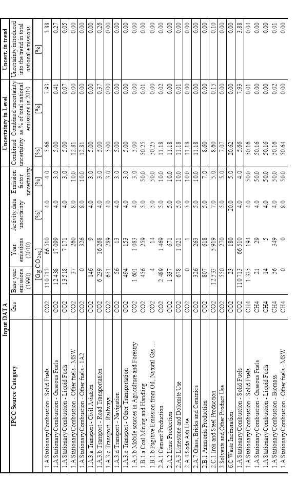
Tab.1‑4 Uncertainty analysis in levels and trend assessments for 2010 (Tier 1), continuation

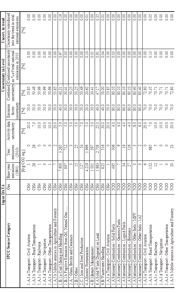
Tab.1‑5 Uncertainty analysis in levels and trend assessments for 2010 (Tier 1), continuation

1.8 General Assessment of Completeness

CRF Table 9 (Completeness) has been used to give information on the aspect of completeness. This part of the text includes additional information. All the categories of sources and sinks included in the IPCC Guidelines are covered. No additional sources and sinks specific to the Czech Republic have been identified. Both direct GHGs as well as precursor gases are covered by the Czech inventory. The geographic coverage is complete.

1.8.1 Notation keys

The sources and sinks not considered in the inventory but included in the IPCC Guidelines are clearly indicated and the reasons for this exclusion are explained. In addition, the notation keys presented below are used to fill in the blanks in all the CRF tables. Notation keys are used according to the UNFCCC guidelines on reporting and review (FCCC/CP/2002/8).

Allocations to categories may differ from Party to Party. The main reasons for different category allocations are different allocations in the national statistics, insufficient information on the national statistics, national methods, and the impossibility of disaggregating the reported emission values.

IE (included elsewhere):

“IE” is used for emissions by sources and removals by sinks of greenhouse gases that have been estimated but included elsewhere in the inventory instead of in the expected source/sink category. Where “IE” is used in the inventory, the CRF completeness table (Table 9) indicates where (in the inventory) these emissions or removals have been included. This deviation from the expected category is explained.

NE (not estimated):

“NE” is used for existing emissions by sources and removals by sinks of greenhouse gases that have not been estimated. Where “NE” is used in an inventory for emissions or removals, both the NIR and the CRF completeness table indicate why the emissions or removals have not been estimated. For emissions by sources and removals by sinks of greenhouse gases marked by “NE”, check-ups are in progress to establish if they actually are “NO” (not occurring). As part of the improvement programme of the inventory, it is planned that these source or sink categories will be either estimated or allocated to “NO”.

Overview of not estimated (NE) categories of sources and sinks and categories included elsewhere (IE) and the relevant explanations are given in CRF Table 9(a).

2 Trends in Greenhouse Gas Emissions

According to the Kyoto Protocol, Czech national GHG emissions have to be 8 % below base year emissions during the five-year commitment period from 2008 to 2012. The Czech Republic is in a good direction to meet its goal.

2.1 Description and Interpretation of Emission Trends for Aggregated Greenhouse Gas Emissions

Tab. 2‑1 presents a summary of GHG emissions excl. bunkers for the period from 1990 to 2010. For CO₂, CH₄ and N₂O the base year is 1990; for F-gases the base year is 1995.

Tab. 2‑1 GHG emissions from 1990-2010 excl. bunkers [Gg CO₂ eq.]

	CO₂^{^[6]}	CH₄⁶	N₂O⁶	HFCs	PFCs	SF₆	Total emissions
	CO₂^{^[6]}	CH₄⁶	N₂O⁶	HFCs	PFCs	SF₆	incl. LULUCF	excl. LULUCF
1990	165097	17914	12865	NO	NO	78	192204.31	195822.25
1991	154604	16277	10932			77	172749.67	181786.95
1992	140228	15339	9804			77	154554.54	165341.47
1993	136191	14420	8644			77	149781.45	159214.31
1994	127173	13575	8534			76	142097.27	149238.34
1995	128158	13398	8821	1	0	75	143131.38	150341.49
1996	132663	13277	8449	101	4	78	146811.26	154431.90
1997	129782	13022	8575	245	1	95	144911.29	151572.13
1998	123403	12574	8452	317	1	64	137680.82	144678.78
1999	115851	11978	8296	267	3	77	129195.79	136350.82
2000	125908	11177	8389	263	9	142	138251.22	145775.46
2001	125669	10887	8557	393	12	169	137694.60	145572.52
2002	122319	10502	8312	391	14	68	133850.87	141483.41
2003	125726	10446	7873	590	25	101	138867.45	144610.10
2004	127245	10156	8506	600	17	52	140255.41	146438.37
2005	127057	10514	8196	594	10	86	139640.50	146326.00
2006	128770	10817	8044	872	23	83	144983.54	148448.20
2007	128790	10471	8093	1606	20	76	148121.44	148848.26
2008	123725	10534	8232	1262	27	47	138889.76	143662.62
2009	115848	10206	7691	1042	27	50	127859.19	134722.30
2010	119866	10413	7477	1503	29	16	133639.37	139157.86
% ^{^[7]}	-29.22	-41.87	-41.88	2046.8 times	240.2 times	-79.12	-30.47	-28.94

Note: Global warming potentials (GWPs) used (100 years time horizon): CO₂ = 1; CH₄ = 21; N₂O = 310; SF₆ = 23 900; HFCs and PFCs consist of different substances, therefore GWPs have to be calculated individually depending on substances

GHG emissions and removals have significantly decreased in the period 1990 – 1994, mainly driven by the economy transition and pursuing major dropdown in heavy industry activities in the country. The fast decrease has stopped around 140000 Gg CO₂eq.and continues fluctuating ever since (see fig. Fig. 2‑1 Total GHG emissions (incl. LULUCF) for the period from 1990-2010 [Gg CO2eq.]). From 2009 to 2010 the total GHG emissions (incl. LULUCF) increased by 4.52 % or 5780.18 Gg CO₂ eq. resulting in total emissions of 133 639.37 Gg CO₂ eq. The increase was caused by CO₂, CH₄, HFC and PFC emissions (raised by 4.9 %; 2.0 %; 44.3 % and 8.4 % respectively) and despite decrease in N₂O and SF₆ emissions (lowered by 2.8 % and 67.3% respectively) compared to previous year. The total GHG emissions and removals in 2010 were 30.47 % below the base year level including LULUCF and 28.94 %, when excluding LULUCF.

In 1989 “then” Czechoslovak economy was one of the centrally planed economies with high level of monopolization. All economic processes were controlled through central planning. For all practical purposes, there was no real market and this situation resulted in an ever depending economic and technological lag which results in high energy and material inefficiency. Since 1989 to the present the economy transformed successfully to a developed market-driven economy. The transformation led to a decline in production, investment in environmental protection, energy efficiency, fuel switch and increased use of renewable energy.

Greenhouse gases emission trend passed between 2007 and 2009 a significant change driven mainly by economic recession. It is noteworthy that in 2009 some of the industrial subsectors reached it’s lowest amounts of emitted GHGs according to the whole reported time-series.

Trend between 2009 and 2010 increased significantly, indicating slight recovery from recesion driven decrease in previous years.

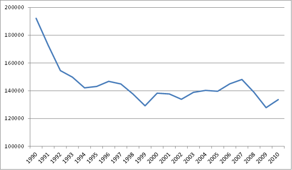
Fig. 2‑1 Total GHG emissions (incl. LULUCF) for the period from 1990-2010 [Gg CO₂eq.]

2.2 Description and Interpretation of Emission Trends by Gas

The major greenhouse gas in the Czech Republic is CO₂, which represents 85.5% of total GHG emissions and removals in 2010, compared to 83.9% in the base year. It is followed by CH₄ (7.8 % in 2010, 9.3 % in the base year), N₂O (5.6 % in 2010, 6.7 % in the base year) and F-gases (1.16 % in 2010, 0.04 % in the base year).

The trend of individual gas emissions is presented in Fig. 2‑2 and Fig. 2‑3 relative to emissions in the respective base years^{^[8]}.

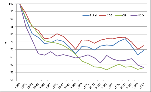
Fig. 2‑2 Trend in CO₂, CH₄ and N₂O emissions 1990-2010 in index form (base year = 100 %)

CO₂

CO₂ emissions have been rapidly decreasing in early 90’s, after 1994 the emissions have kept at aprox. 70-75 % of the amount produced in 1990. Between 2007 and 2009 emissions of CO₂ dropped to it’s lowest value among the whole reported period. Inter-annual increase in CO₂ emissions (excl. LULUCF) from 2009 to 2010 by 3.3 % results the total decrease to 28.9 % from 1990 to 2010 (30.5 % decrease incl. LULUCF). Quoting in absolute figures, CO₂ emissions and removals decreased from 165 097 to 119 866 Gg CO₂eq. in the period from 1990 to 2010, mainly due to lower emissions from the 1 Energy category (mainly 1A2 Manufacturing Industries & Construction, 1A4A Commercial / Institutional and 1A4B Residential).

The main source of CO₂ emissions is fossil fuel combustion; within the 1A Fuel Combustion category, 1A1 Energy Industry and 1A2 Manufacturing Industries & Construction sub-categories are the most important. CO₂ emissions increased remarkably between 1990 and 2007 from the 1A3 Transport category from 7 767 to 17 448 Gg CO₂.

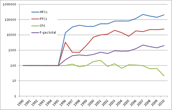
Fig. 2‑3 Trend in HFCs, PFCs (1995 – 2010) and SF₆ (1990 – 2010) actual emissions in index form (base year = 100 %)

Fig. 2‑4 Percentual share of GHGs (Y-axis begins at 80% - part of energy share is hidden)

CH₄

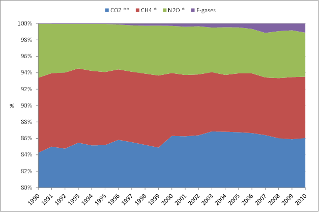
CH₄ emissions share decreased almost steadily during the period from 1990 to 2004, slightly increase from 2004 to 2006 and decrease by 7.9 % between 2006 and 2009 recently CH₄ increased slightly resulting the overall share at 7.79 %. In 2010 CH₄ emissions were 41.87 % below the base year level, mainly due to lower contribution of 1B Fugitive Emissions from Fuels and emissions from 4 Agriculture and despite increase from the 6 Waste category.

The main sources of CH₄ emissions are 1B Fugitive Emissions from Fuels (solid fuel), 4 Agriculture (4A Enteric Fermentation and 4B Manure Management) and 6 Waste (6A Solid Waste Disposal on Land and 6B Waste-water Handling).

N₂O

N₂O emissions strongly decreased from 1990 to 1994 by 33.9 % over this period and then shows slow decreasing trend with inter-annual fluctuation. N₂O emissions decreased between 1990 and 2010 from 12 865 to 7 477 Gg CO₂eq. In 2010 N₂O emissions were 41.88 % below the base year level, mainly due to lower emissions from 4 Agriculture and 2B. Chemical Industry and despite increase from the 1A3 Transport category.

The main source of N₂O emission is category 4D Agricultural Soils (others less important sources are 1A Fossil Fuel Combustion and 2 Industrial Processes - 2B Chemical Industry).

HFCs

HFCs actual emissions increased remarkably between 1995 and 2010 from 0.7 to 1 503.4 Gg CO₂eq. Emissions of HFCs have been increasing since the base year 1995 (except 2008 and 2009), when they were started to use. In 2010, HFCs emissions were more than 2000-times higher than in the base year 1995.

The main sources of HFCs emissions are Refrigeration and Air Conditioning Equipment.

PFCs

PFCs actual emissions show very similar trend as HFCs emissions to the year 2009 as they increased remarkably between 1995 and 2010 from 0.12 to 29.4 Gg CO₂eq. In 2010, PFCs emissions are over 200 times higher than in the base year 1995. HFCs and PFCs have not been imported and used before 1995.

The main sources of PFCs emissions are Semiconductor Manufacture, Refrigeration and Air Conditioning Equipment.

SF₆

SF₆ actual emissions in 1995 amounted for 75.2 Gg CO₂eq. Between 1995 and 2010 they inter annually fluctuated with maximum of 168.7 Gg CO₂eq. in 2001 and minimum of 47.0 Gg CO₂ eq. in 2008. In 2010, they reached whole time-span minimum of 16.22 Gg, the level was below the base year level by 79.1 %.

The main sources of SF₆ emissions are Electrical Equipment; Semiconductor Manufacture and Filling of Insulate Glasses.

2.3 Description and Interpretation of Emission Trends by Category

Tab. 2‑2 presents a summary of GHG emissions by categories for the period from 1990 to 2010:

Category 1. Energy

Category 2. Industrial Processes

Category 3. Solvent and Other Product Use

Category 4. Agriculture

Category 5. Land Use, Land-Use Change and Forestry

Category 6. Waste

The dominant category is the 1 Energy category, which caused for 86.2% of total GHG emissions in 2010 (81.7 % in 1990) excluding LULUCF, followed by the categories 2 Industrial Processes and 4 Agriculture, which caused for 9.0 % and 5.8 % of total GHG emissions in 2009, (10.2 % and 8.2 % in 1990, resp.) 6 Waste category covered 2.7 %, 3 Solvent and Other Product Use 0.4 % and 5 LULUCF category removed 5518Gg CO₂eq.

The trend of GHG emissions by categories is presented in Fig. 2‑5 (relative to the base year).

Tab. 2‑2 Summary of GHG emissions by category 1990-2010 [Gg CO₂ eq.]

	1 Energy	2 IP	3 Solvents	4 Agri	5 LULUCF	6 Waste
1990	157048	19603	765	15733	-3618	2673
1991	149761	14619	728	13956	-9037	2723
1992	133657	16069	691	12191	-10787	2733
1993	132205	12923	651	10686	-9433	2750
1994	122009	13856	616	9898	-7141	2859
1995	123775	13188	596	9875	-7210	2908
1996	127529	13893	587	9540	-7621	2882
1997	123796	14847	585	9377	-6661	2967
1998	117260	14850	580	8977	-6998	3012
1999	111588	12103	578	9053	-7155	3029
2000	119801	13561	569	8786	-7524	3058
2001	120105	12886	550	8919	-7878	3113
2002	116449	12546	540	8706	-7633	3242
2003	118957	13672	525	8127	-5743	3329
2004	119865	14274	519	8502	-6183	3277
2005	121400	12980	514	8135	-6686	3297
2006	122414	14156	513	8013	-3465	3351
2007	121559	15265	512	8179	-727	3333
2008	117196	14085	515	8374	-4773	3492
2009	111587	11175	506	7926	-6863	3529
2010	115205	12061	503	7777	-5518	3612
%[9]	3.24	7.93	-0.68	-1.88	-19.59	2.36
%[10]	26.64	38.47	34.28	50.57	52.53	-35.11

Fig. 2‑5 Emission trends in 1990-2010 by categories in index form (base year = 100)

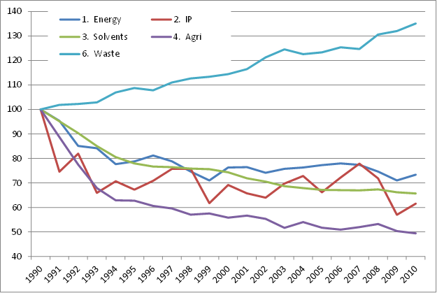
Fig. 2‑6 Percentual share of GHG emissions by categories (y-axis begins at 80% - part of energy share is hidden)

Energy (IPCC Category 1)

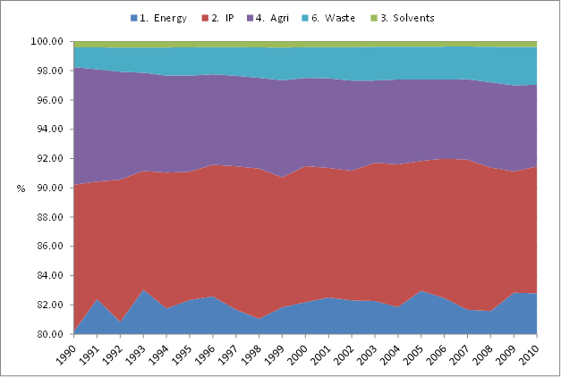
The trend for GHG emissions from 1 Energy category shows decreasing trend of emissions. They strongly decreased from 1990 to 1994 and than fluctuated by 2002. After 2002 they stayed relatively stable by 2007. In the period 2002 – 2007 emissions stayed from around 120 000 Gg CO₂eq. Total decrease between 1990 and 2009 is 26.64 %. Between 2009 to 2010 emissions from category 1 Energy slightly increased by 3.24 %.

From the total 115 205 Gg CO₂eq. in 2010 96.3 % comes from 1A Fuel Combustion, the rest are 1B Fugitive Emissions from Fuels (mainly solid fuels). 1B Fugitive Emissions from Fuels is the largest source for CH₄, which represented around 38.2 % of all CH₄ emissions in 2010. 44 % of all CH₄ emissions in 2010 originated from Energy category.

CO₂ emission from fossil fuel combustion (category 1 Energy) is the main source of emissions in CR inventory with a share of 81.70 % in national total emissions (incl. LULUCF). CO₂ contributes for 95.04 % to total GHG emissions from 1 Energy category, CH₄ for 4.0 % and N₂O for 1.0 % in 2010.

Industrial Processes (IPCC Category 2)

GHG emissions from the 2 Industrial Processes category fluctuated during the period 1990 to 2010. In early 90’s emissions decreased very rapidly, then fluctuated with minimum in 1999 and subsequently fluctuated with total minimum in 2009 (successful implementation abatement technology). Between 1990 and 2010 emissions from this category decreased by 38.47%. In 2010 emissions amounted for 12 061 Gg CO₂eq.

The main categories in the 2 Industrial Processes category are 2C Metal Production (49.1 %), 2A Mineral Products (28.4 %), 2B Chemical Industry (5.1 %) and 2F Consumption of Halocarbons and SF₆ (12.8 %) of the sectoral emissions in 2010.

The most important GHG of the 2 Industrial Processes category was CO₂ with 82.6 % of sectoral emissions, followed by F-gases (12.1 %), N₂O (3.9 %), CH₄ (0.7 %).

Solvent and Other Product Use (IPCC Category 3)

In 2010, 0.4 % of total GHG emissions (502.68 Gg CO₂eq.) arose from the 3 Solvent and Other Product Use category. Emissions generally decreased steadily in the period from 1990 to 2010, but has steadily kept it’s 0.4% share over all the years. In 2010 GHG emissions from 3 Solvent and Other Product Use were -34.3 % below the base year level. 53.7 % of these emissions were CO₂, N₂O emissions contributed by 46.3 %.

Agriculture (IPCC Category 4)

GHG emissions from the category 4 Agriculture decreased relatively steadily near over the all period from 1990 to 2003 and then fluctuated. In 2010 emissions reached the minimum level. In 2010 emissions were by 50.6 % below the base year level.

They amounted 7 777 Gg CO₂eq. in 2010 which corresponds to 5.8 % of national total emissions (excluding LULUCF). The most important sub-category agricultural soils (N₂O emissions) contributed by 60.4 % to sectoral total in 2010, followed by the enteric fermentation (CH₄ emissions, 25.7 %) and manure management (CH₄ and N₂O emissions, 5.1 % and 8.8 % respectively).

4 Agriculture is the largest source for N₂O and second largest source for CH₄ emissions: 72 % of all N₂O emissions and 23 % of all CH₄ emissions in 2010 originated from this category.

Land Use, Land-Use Change and Forestry (IPCC Category 5)

GHG removals from the 5 Land Use, Land-Use Change and Forestry category vary through the whole time series with minimum of 730 Gg CO₂eq. in 2007 and maximum 10 794 CO₂eq. in 1992. In 2010 removals were by 52.53 % above the base year level.

Emissions and removals amounted to -5518.5 Gg CO₂eq. in 2010, which corresponds to - 4.1 % to national total emissions. Emissions and removals are calculated from all categories and according to GPG for LULUCF; IPCC 2003.

LULUCF category is the largest sink for CO₂. CO₂ removals from this category amounted to 5952.63 Gg in 2010, CH₄ emissions amounted for 128.21 Gg CO₂eq., N₂O to 19.41 Gg CO₂eq.

Waste (IPCC Category 6)

GHG emissions from 6 Waste category slowly increased during the whole period. In 2010 emissions amounted for 3611.8 Gg CO₂eq., which is 35.1 % above the base year level. The increase of emissions is mainly due to higher emissions of CH₄ from 6A Solid Waste Disposal on Land (and partly due to increase of N₂O emissions from 6B Waste-water Handling), which is the most important category. As a result of CH₄ recovery systems installed in 6B Waste-water Handling emissions decreased in this category by 27 % compared to the base year. The share of category 6 Waste in total emissions was 2.7 % in 2010 (excluding LULUCF).

The main source is solid 6A Solid Waste Disposal on Land, which caused for 75.0 % of sectoral emissions in 2010, followed by 6B Waste-water Handling (CH₄ - 14.3 % and N₂O - 5.7 %) and 6C Waste Incineration (CO₂ – 5.0 %; CH₄ - negligible and N₂O - 0.1 %).

89.3 % of all emissions from Waste category are CH₄ emissions; CO₂contributes by 5.0 % and N₂O by 5.8 %.

2.4 Description and Interpretation of Emission Trends of Indirect Greenhouses Gases and SO₂

Emission estimates for NO_x, CO, NMVOC and SO₂ are also reported in the CRF. The following chapter summarizes the trends for these gases.

A detailed description of the methodology used to estimate these emissions was provided in the Czech Informative Inventory Report (IIR) 2010, Submission under the UNECE / CLRTAP Convention, which was published in March 2012.

Tab. 2‑3 presents a summary of emission estimates for indirect GHGs and SO₂ for the period from 1990 to 2010 and the National Emission Ceilings (NEC) as set out in the 1999 Gothenburg Protocol to Abate Acidification, Eutrophication and Ground-level Ozone. These reduction targets should be met by 2010 by Parties to the UNECE / CLRTAP Convention signed this Protocol.

Emissions of indirect greenhouse gases decreased from the period from 1990 to 2010 (NMVOC by 51.9 %, CO by 57.5 % and NO_x by 67.6 %). SO₂ emissions decreased by 90.9 % compared to 1990 level.

Tab. 2‑3 Emissions of indirect GHGs and SO₂ 1990-2010 [Gg]

	NO_x	CO	NMVOC	SO₂
1990	742.4	1071.8	311.3	1875.5
1991	732.2	1157.6	273.0	1772.2
1992	708.3	1162.9	257.5	1559.1
1993	690.8	1194.6	233.0	1468.9
1994	450.9	1075.8	255.3	1290.2
1995	430.2	933.5	215.3	1095.3
1996	446.7	966.7	265.2	934.5
1997	470.8	982.7	271.9	980.8
1998	414.2	814.0	267.1	442.2
1999	391.1	728.0	247.2	268.9
2000	396.7	681.5	244.3	264.4
2001	332.9	688.7	219.9	250.9
2002	319.5	589.2	202.9	237.4
2003	325.8	632.4	203.3	232.1
2004	333.6	624.4	198.5	227.2
2005	279.2	558.0	181.7	218.6
2006	283.8	542.1	178.6	211.2
2007	285.9	584.3	174.0	217.0
2008	262.8	498.4	165.7	174.3
2009	252.8	454.1	151.1	173.5
2010	240.8	455.1	149.9	170.2
%[11]	-67.6	-57.5	-51.9	-90.9
NEC[12]	286	-	220	283

NO_x

NO_x emissions decreased from 742 to 241 Gg during the period from 1990 to 2010. In 2010 NO_x emissions were 67.6 % below the 1990 level. Nearly 99 % of NO_x emissions originate from 1 Energy, mainly subsectors 1A1 Energy Industries, 1A3 Transport (road), 1A2 Manufacturing Industries and Construction and 1A5 Other.

CO

CO emissions decreased from 1,071 to 455 Gg during the period from 1990 to 2010. In 2010 CO emissions were 57.5 % below the 1990 level. In 2010, approximately 86 % of total CO emissions originated from 1 Energy (subsectors 1A3 Transport, 1A2 Manufacturing Industries and Construction and 1A4 Other Sectors (Commercial / Institutional, Residential, Agriculture / Forestry / Fisheries), followed by 5A Forest land (11.0 %) and Industrial Processes (2.6 %).

NMVOC

NMVOC emissions decreased from 311 to 150 during the period from 1990 to 2010. In 2010 NMVOC emissions were 51.9 % below the 1990 level. There are two main emission source categories, first is 3 Solvent and Other Product Use (50 % of the national total) and second is 1 Energy (40 % - mainly subsectors 1A3 Transport (20 %), and 1A4 Other Sectors (Commercial / Institutional, Residential, Agriculture / Forestry / Fisheries) 10 %).

SO₂

SO₂ emissions decreased from 1 876 to 169 Gg during the period from 1990 to 2010. In 2009 SO₂ emissions were 87 % below the 1990 level. In 2010, 99.6 % of total SO₂ emissions originated from 1 Energy mainly subsectors 1A1 Energy Industries, 1A2 Manufacturing Industries and Construction and 1A4 Other Sectors (Commercial / Institutional, Residential, Agriculture / Forestry / Fisheries)).

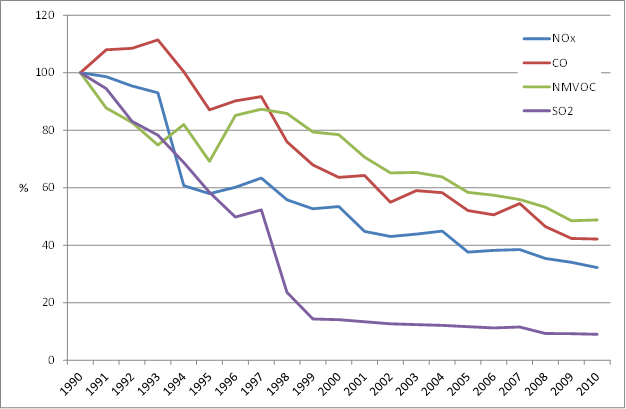
Fig. 2‑7 Emissions of indirect GHGs and SO₂ 1990 – 2010

2.5 Description and Interpretation of Emission Trends for KP-LULUCF inventory

Sinks from Forest Management dominate the emissions and removals estimates of the KP LULUCF activities (see Tab. 2‑4). They were positively affected by the absence of disturbances requiring sanitary logging, which significantly reduced sinks in 2007 and partly also in 2008.

Tab. 2‑4 Summary of GHG emissions and removals for KP LULUCF activities [Gg CO₂ eq.]

	Article 3.3 activities		Article 3.4 activities
	Afforestration and Reforestration	Deforestation	Forest Management*	Cropland Management	Grazing Land Management	Revegetation
2008	-272.0	160.2	-4 404.0 / -4 404.0	NA	NA	NA
2009	-294.7	170.2	-6 441.1 / -5 866.7	NA	NA	NA
2010	-322	207	-5 237.4 / -5 096.0	NA	NA	NA

*) Net emissions or removals / accounting quantity

3 Energy (CRF Sector 1)

Zaoblený obdélník: Provisions of this chapter have been partially updated due to UNFCCC centralised review in September 2012. Body of the chapter below remained unchanged. For details of resubmission changes please see chapter ES 4.2 above.

The energy sector in the Czech Republic is mainly driven by the combustion of fossil fuels in stationary and mobile sources; however fugitive emissions must also be considered. The two main categories are 1A Fossil Combustion and 1B Fugitive Emissions from Fuels.

Activity data for treating the whole sector are based on the energy balance of the Czech Republic prepared by the Czech Statistical Office. Data from the energy balance form the basic framework for processing greenhouse gas emissions from combustion in stationary and mobile sources. Greenhouse gas emissions from stationary sources are calculated from the activity data and the emission factors. CO₂ emissions from mobile sources are calculated from the emission factors, while data on CH₄ and N₂O emissions are calculated using the special model developed by Transport research centre (CDV).

Processing of the activity data is based on the total energy balance of the Czech Republic. The energy balance is prepared by CzSO, and is divided into chapters for solid fuels, liquid fuels, natural gas, renewable energy sources and production of heat and electrical energy. Information on the energy balance forms the basis for preparing a database of activity data in the Reference and Sectoral Approaches. The Reference Approach is based on data from the source part of the energy balance; the Sectoral Approach involves processing of data on fuel consumption in a structure corresponding to the requirements of the IPCC categorization.

Inventories of CO₂, CH₄ and N₂O emissions are performed using a different procedure in subsector 1A3 Transport and in the other subsectors: combustion of fuels in stationary sources (1A1, 1A2, 1A4) and other mobile sources (1A5). The CDV model is used for mobile sources in subsector 1A3 Transport. A calculation procedure based on the activity data and on the country-specific or default emission factors are used for the other subsectors. Another procedure is used for category 1A1a – Other Fuels, which contains Waste Incineration for energy purposes. Detailed description please see in chapter 3.3.1.1 1A1a Public electricity and heat production.

Fugitive emissions in sector 1B are determined by calculation from activity data and country-specific or default emission factors. The activity data are obtained from the sector statistics and annual targeted surveys.

3.1 Overview of sector 1A

Combustion processes included in category 1A make a decisive contribution to total emissions of greenhouse gases. Almost all emissions of carbon dioxide, with the exception of decomposition of carbonate materials, occurring, e.g., in cement production, are derived from the combustion of fossil fuels in stationary and mobile sources. Consequently, the greatest attention is paid in the IPCC Guidelines (IPCC, 1997) to inventories of emissions from these categories.

On the whole, 9 key sources have been identified in sector 1A, the most important of which are the first 3 in Table 3.1. This group of sources contributes 71.9 % to total greenhouse gas emissions (without LULUCF).

It is apparent from the table that the first three categories are of fundamental importance for the level of greenhouse gas emissions in the Czech Republic and, of these, the combustion of solid fuels constitutes a decisive source. This consists primarily in the combustion of solid fuels for the production of electricity and supply of heat. Another important category consists in the combustion of liquid fuels in the transport sector and the combustion of Natural Gas has approximately the same importance. This corresponds mostly to the direct production of heat for buildings in the private and public sector and for households. Consequently, increased attention is paid to it.

The results of the inventory, including the activity data, are submitted in the standard CRF format. For direct greenhouse gases, the consumption of fuels and “implied” emission factors are also given. However, for stationary sources, the fuel consumption is given in the CRF format in aggregated structure, i.e. as solid, liquid and gaseous fuels according to IPCC definition. All the CRF tables in sector 1A were appropriately completed for the entire required time interval of 1990 to 2010.

Tab. 3‑1 Overview of key categories in Sector 1A (2010)

Category		Character of category	Gas	% of total GHG*
1A	Stationary Combustion - Solid Fuels	KC (LA, TA, LA, TA)	CO₂	47.8
1A	Stationary Combustion - Gaseous Fuels	KC (LA, TA, LA, TA)	CO₂	12.3
1A3b	Transport - Road Transportation	KC (LA, TA, LA, TA)	CO₂	11.7
1A	Stationary Combustion - Liquid Fuels	KC (LA, TA, LA, TA)	CO₂	5.2
1A5b	Mobile sources in Agriculture and Forestry and Other	KC (LA, LA*)	CO₂	0.8
1A3b	Transport - Road Transportation	KC (LA, TA, TA*)	N₂O	0.5
1A	Stationary Combustion – Other Fuels (1A2)	KC (TA, TA*)	CO₂	0.2
1A	Stationary Combustion - Biomas	KC (TA, TA*)	CH₄	0.2
1A	Stationary Combustion – Solid Fuels	KC (TA, TA*)	CH₄	0.1

* assessed without considering LULUCF

KC: key category, LA, LA*: identified by level assessment with and without considering LULUCF, respectively

TA, TA*: identified by trend assessment with and without considering LULUCF, respectively.

In 2009, the Expert Review Team (ERT) introduced the requirement of unification of the activity data for the Energy sector with the data that CzSO reports in its official questionnaires for IEA – EUROSTAT – UNECE (FCCC/ARR/2009/CZE, Section 41). Unification of the data is considered to be important to facilitate control of the activity data employed in preparing the emission balance in the ENERGY sector. The same requirement was also introduced during the in-country review in August/September 2011 (FCCC/ARR/2011/CZE, Section 73) in Prague. This requirement was accepted in the 2011 submission and the activity data were modified according to these questionnaires for the time series from 1995. In this year’s submission, data from the questionnaires, provided by CzSO in December 2011, were used for 2010.

This step represents substantial progress in refinement of the activity data.

In 2010, there was a further expansion of cooperation with CzSO. An internal workshop was held in August of 2010, at which, in addition to the workers of the responsible team and the coordination workplace (CHMI), representatives of CzSO, the Ministry of the Environment and Ministry of Industry and Trade also participated. The meeting included discussion of the methodology for conversion of data from the structure of the IEA – EUROSTAT questionnaires to the structure required for drawing up activity data in the Sectoral and Reference Approaches. Simultaneously, suggestions were made for expanding cooperation between the responsible team of NIS and CzSO. In connection with these suggestions, a meeting was held between the Ministry of the Environment and CzSO with participation by representatives of the responsible team and NIS coordinator. This meeting led to an addendum to the original agreement on cooperation between CHMI and CzSO. The addendum defines the terms and means of submitting data for preparation of the emission inventories of greenhouse gases in the ENERGY sector and performance of subsequent control procedures. Unfortunately a workshop similar to the one in 2009 was not held in 2011. Instead, a number of meetings were held with CzSO, where current problematic issues were resolved. These meetings were just on at the KONEKO - CzSO level, but they contributed positively to the preparation of this submission.

Since 2003, the balance of fuel consumption has been supplemented by consumption of Other Fuels and the corresponding greenhouse gas emissions. As this consists exclusively of consumption in cement-plant furnaces, this consumption and emissions were included in category 1A2f.

The CzSO Questionnaires (IEA/OECD, Eurostat, UN Questionnaires) represent the official reports of the Czech Republic, for international purposes, on the consumption of the individual kinds of fuel. They consist in a set of data on liquid, solid and gaseous fuels in independent datasets. They contain source and consumption parts of the energy balance in a structure that permits processing of activity data in the CRF structure. The use of these reports is advantageous especially because they provide a very similar data structure to CRF. The transition from the final CzSO balance to the use of these reports does not affect the consistency of the time series, as the same data are involved.

The overall energy balance for 2010 is given in Annex 4.

The fact that only CzSO data were employed constitutes a substantial improvement in the methodology of processing activity data. The data of other institutions and organizations were used for control. These consisted in documents of the Ministry of Industry and Trade (MIT), the Czech Association of the Petroleum Industry (CAPPO), Czech Gas Association (CGA) and other organizations.

Emissions Trends

CO₂ emissions from the 1A sector decreased by 25.2 % from 146 Tg CO₂ in 1990 to 109 Tg CO₂ in 2010.

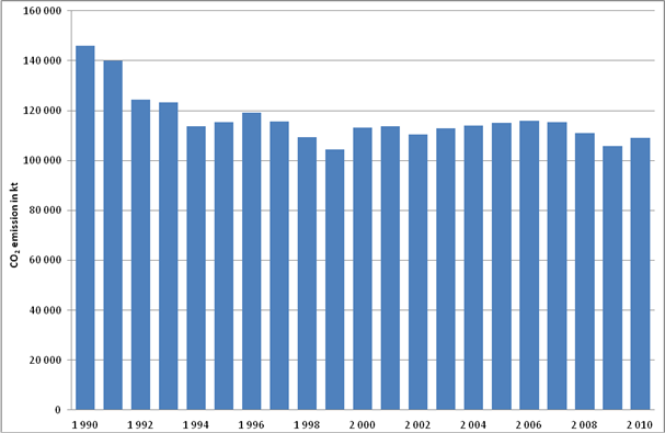
Fig. 3‑1 Trend total CO₂ (Sectoral Approach) in period 1990 – 2010

Tab. 3‑2 Emissions of greenhouse gases and their trend from 1990 – 2010 from IPCC Category 1A Energy

	CO₂ [Gg]	CH₄ [Gg]	N₂O [Gg]
1990	146354	474	2368
1991	140464	409	2251
1992	124831	389	2111
1993	123753	371	2128
1994	114026	349	2088
1995	115830	344	2306
1996	119650	339	2433
1997	116049	332	2467
1998	109787	319	2518
1999	104740	288	2552
2000	113561	256	2766
2001	114143	241	2917
2002	110865	221	3059
2003	113334	218	3376
2004	114355	210	3573
2005	115431	229	3718
2006	116152	242	3780
2007	115625	225	3923
2008	111305	224	3828
2009	105994	211	3743
2010	109454	218	3768
Trend 1990/2010	-25.2 %	-54%	59.1 %

Emission trends by subcategories

The individual subsectors have different contributions to trends in emissions. Fig. 3.2 illustrates the trends in emissions on the example of CO₂ emissions.

The greatest increase in emissions was recorded in subsector 1A3 Transport between 1990 and 2007, when emissions increased by 145%. In absolute values, this corresponded to an increase from 7.5 Tg CO₂ in 1990 to 18.5 Tg in 2007. A slight decrease has been apparent since 2008, by 1.7 Tg in 2010. Emissions from subsector 1A1 Energy Industries were practically constant with slight fluctuations over the entire period; the greatest reduction occurred in subsectors 1A2 and 1A4 from 46.6 and 32.3 Tg CO₂ in 1990 to 23.6 and 11.7 Tg CO₂ in 2010, respectively.

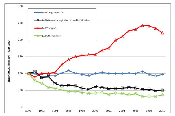
Fig. 3‑2 Share of CO₂ emissions from 1990 - 2010 in individual sub-sectors

Tab. 3‑3 Total GHG emissions in [Gg CO₂ equivalent] from 1990 – 2010 by sub categories of energy.

	1	1A	1A1	1A2	1A3	1A4	1A5	1B	1B1	1B2
1990	157 048	148 090	58 008	46 885	7 767	33 803	1 628	8 958	8 056	902
1991	149 761	141 854	57 697	49 442	6 949	26 333	1 432	7 906	7 136	770
1992	133 657	126 128	51 554	41 349	7 820	24 063	1 342	7 528	6 818	710
1993	132 205	124 881	53 806	42 254	7 746	19 778	1 297	7 324	6 631	693
1994	122 009	115 045	53 991	32 814	8 098	18 835	1 306	6 964	6 284	679
1995	123 775	116 929	59 056	29 587	9 896	17 179	1 211	6 846	6 165	681
1996	127 529	120 811	62 826	30 022	11 022	15 781	1 159	6 718	5 982	737
1997	123 796	117 200	58 748	29 605	11 747	15 891	1 209	6 595	5 871	725
1998	117 260	110 851	56 360	26 541	12 001	14 659	1 290	6 409	5 647	762
1999	111 588	105 727	54 217	24 445	12 225	13 567	1 273	5 861	5 114	746
2000	119 801	114 637	57 809	29 086	12 366	14 114	1 262	5 164	4 455	709
2001	120 105	115 260	59 720	26 945	13 253	14 122	1 220	4 845	4 178	667
2002	116 449	111 942	58 031	26 184	13 880	12 681	1 166	4 507	3 814	693
2003	118 957	114 558	57 849	25 802	15 760	14 064	1 084	4 400	3 763	637
2004	119 865	115 659	57 746	26 590	16 572	13 619	1 132	4 207	3 614	592
2005	121 400	116 788	58 594	27 000	17 946	12 129	1 119	4 612	3 908	704
2006	122 414	117 592	58 063	26 730	18 282	13 419	1 098	4 822	4 107	715
2007	121 559	117 094	61 636	24 323	19 236	10 788	1 110	4 466	3 751	715
2008	117 196	112 727	56 393	24 876	19 075	11 225	1 159	4 469	3 814	655
2009	111 587	107 442	53 702	23 201	18 501	10 896	1 143	4 145	3 450	695
2010	115 205	110 954	56 251	23 807	17 448	12 340	1 108	4 251	3 525	726
*Total Trend*	-26.6%	-25.1%	-3.0%	-49.2%	124.7%	-63.5%	-31.9%	-52.5%	-56.2%	-19.5%
*1990 - 2010*	-26.6%	-25.1%	-3.0%	-49.2%	124.7%	-63.5%	-31.9%	-52.5%	-56.2%	-19.5%

Table 3.3 gives the trends in GHG emissions in the individual subcategories of the Energy sector. It is apparent from the table that there was a considerable increase in the area of transport and a substantial reduction in the processing industry and in households, as well as the areas of Commercial and Institutional and Agriculture, Forestry and Fishing.

3.2 Fuel combustion (1A)

Combustion of fuels is in CRF divided into the individual subsectors prescribed by the IPCC methodology. The fuel consumption in the individual subsectors yields the activity data for subsequent calculation of greenhouse gas emissions. The fuel consumption is taken from the energy balance of the

Czech Republic and is transformed to the IPCC structure. Transformation of data is described in Chapter 3.2.6 under the descriptions of the individual subsectors. Consumption of the other kinds of fuels (Other fuels) was taken from the national ETS system (ETS, 2011, http://www.svcement.cz/).

According to IPCC methodology (IPCC, 1997), carbon dioxide emissions are calculated in two ways: Sectoral and Reference Approach.

3.2.1 Sectoral Approach

The Sectoral Approach. This method is considerably more demanding than Reference Approach in relation to input data and requires information on fuel consumption according to kind in the individual consumer sectors. It has an advantage in the possibility of analyzing the structure of the origin of emissions. As the emission factors employed are specific for each kind of fuel burned, calculations using this method should be more exact.

In Sectoral Approach are calculated CO₂ emissions in sectors

· 1A1 Energy industries

· 1A2 Manufacturing Industries and Construction

· 1A3 Other transportation (combustion of part of Natural Gas during its transport in compressors)

· 1A4 Other sectors – excl. mobile sources in the Agriculture/Forestry/Fishing sector

· 1A5 Other – other mobile sources not included elsewhere

In the Sectoral Approach, CO₂ emissions are derived from the consumption of the individual kinds of fuel in the individual subcategories using emission and oxidation factors.

3.2.2 Reference Approach

The Reference Approach is calculated on the basis of total domestic consumption of the individual fuels. This relatively simple method is based on the assumption that almost all the fuel consumed is burned in combustion processes in energy production. It does not require a large amount of input activity data and the basic values of the sources included in the national energy balance and some supplementary data are sufficient. It provides information only on total emissions without any further classification in the consumer sector. The emission factors are related to those kinds of fuel that enter domestic consumption at the level of sources, without regard to specific kinds of fuel burned in the consumer part of the energy balance. Thus, for liquid fuels, this means that the emissions are determined practically only on the basis of domestic petroleum (crude oil) consumption.

In the previous submission, data on production of Other Fuels was accidentally included in the

Reference Approach in CRF (the “Production” line for 2003 - 2010). These data were removed from the current submission.

3.2.3 Comparison of the Sectoral Approach with the Reference Approach

The resulting emissions are determined by the Sectoral Approach (SA), while the Reference Approach (RA) is used for control. Comparison of both approaches is given in the Annex 4. It follows from the analysis in this Annex that the differences in the overall results from the two methods are insignificant.

3.2.4 International bunkers fuels

In the Czech Republic, this corresponds only to the storage of Kerosene Jet Fuel for international air transport since the Czech Republic does not have an ocean fleet.

Basic activity data are available in the CzSO energy balance (CzSO, 2011). Table 3.4 gives the amount of stored Kerosene Jet Fuel.

Tab. 3‑4 Kerosene Jet Fuel in international bunkers

Year	1990	1991	1992	1993	1994	1995	1996	1997	1998	1999	2000
[TJ/year]	7 197	5 919	6 856	5 706	7 112	7 664	5 789	6 676	7 880	7 417	8091
Year	2001	2002	2003	2004	2005	2006	2007	2008	2009	2010
[TJ/year]	8 599	7 424	9 983	12 835	13 338	13 833	14 512	15 361	14 046	13155

3.2.5 Feedstocks and non-energy use of fuels

The energy balance of the Czech Republic encompasses a number of items that contain information on the consumption of fuel used as a raw material for production of other kinds of fuels. This corresponds mainly to petroleum, which is given in the source part of the energy balance; however, its entire volume undergoes transformation to other kinds of fuel, so that petroleum itself does not enter the fuel balance as activity data in CRF for the calculation of greenhouse gases.

In the energy balance structure, improvement of fuels is included in the Transformation Sector chapter. This chapter contains information on the amounts of fuel used for the production of electrical energy and heat and simultaneously also for conversion (improvement) of the original fuels to other kinds (e.g. Coke, Briquettes, Coal Gases, etc.). Fuels from the Transformation Sector chapter employed for the production of electrical energy and heat are transferred directly to the CRF structure as activity data to sector 1A1 – Energy Industry. Fuels and other items in the Transformation Sector chapter need to be seen as raw materials for production of the derived fuels and this amount from the energy balance does not enter the CRF structure as activity data, as no greenhouse gases are formed from them in this stage.

The classification in the energy balance in the Transformation sector is dependent on the kind of fuel.

The following survey gives those items of the Transformation sector that correspond to raw material inputs into the improvement processes.

Tab. 3‑5 Transformation sector for Solid and Liquid fuels

Solid fuels	Liquid fuels
Transformation Sector	Transformation Sector
Patent Fuel Plants (Transformation)	Gas Works (Transformation)
Coke Ovens (Transformation)	For Blended Natural Gas
BKB Plants (Transformation)	Coke Ovens (Transformation)
Gas Works (Transformation)	Blast Furnaces (Transformation)
Blast Furnaces (Transformation)	Patent Fuel Plants (Transformation)
Coal Liquefaction Plants (Transformation)	Non-specified (Transformation)

Natural Gas is not currently used as a raw material in the Czech Republic. Things were different at the beginning of the 1990’s, when Natural Gas was used as a raw material in the production of Coal Gas.

Biofuels are not used in transformation processes.

The decomposition of Petroleum also leads to a number of products that are not intended for energy use. This corresponds to the production of plastics, Lubrication Oils and other Lubricants, solvents for production of coatings and other uses in the Solvent Use sector, production of Bitumen, etc.

Part of these material fluxes become waste, while part is used up irreversibly and this carbon must be considered to be carbon stored permanently.

Naphtha - another part of fossil carbon is used as raw material for the manufacture of plastics. Plastics end up in waste incineration plants or in landfills. In incineration plants, the carbon in the plastics is converted to CO₂. In managed landfills, plastics very slowly decompose through biochemical processes. For detailed explanations please see relevant chapter for Other Fuels (1A1a).

However, part of plastics stores carbon from petrochemical raw materials for a long time. At the beginning of the monitored period, the fraction of carbon stored for naphtha was expertly estimated at 50 %. This value was obtained by expert estimate of a sectoral expert.

The remaining 50 % of carbon was considered to oxidize to CO₂. Recently, plastics have been increasingly recycled. The recycled material obtained is used to manufacture products with considerably long lifetimes. In 2004 was decided to increase the fraction of carbon stored 50 % to the value given in IPCC methodology. The fraction of stored carbon has been gradually increased from a value of 50 % to a value of 80 %. The value of 80% is given in Revised 1996 IPCC methodology (section 1.37). The following survey depicts the gradual increase.

Tab. 3‑6 Naphtha - fraction of stored carbon

1990 - 2003	2004	2005	2006	2007	2008	2009	2010
0.5	0.6	0.7	0.8	0.8	0.8	0.8	0.8

Starting in 2007, a constant value of 80 % is used in subsequent years.

Lubricating oils and other lubricants are not produced primarily as energy production materials.

However, part of the oils is returned to the energy system after the end of their lifetimes as lubricants.

They are then converted to alternative fuels and burned. The CRF structure specifies 50 % recovery as fuels over the entire time series from 1990. Value of 50% is given in Revised 1996 IPCC methodology.

Asphalt (Bitumen) is a product of petroleum processing. As it is used primarily for treating the surfaces of roadways, its entire volume must be considered to be permanently stored carbon that is100% fixed over the entire time series.

Coal Tars are utilized primarily as a raw material for the production of soot as a filler for rubber for production of tires. Part of the Tars is used as additive fuel in energy-production installations for production of electricity and heat. This part has been reported separately in the energy balance since 2003. This permits estimation of the ratio between Tar for energy-production and other uses. Up until 2002, the fraction of Tars for non-energy use was estimated at 75%; since 2003, the fraction has been determined on the basis of information from the CzSO – EUROSTAT – IEA questionnaires (CzSO, 2011) in the following way:

Tab. 3‑7 Coal Tars - fraction of non-energy use

2003	2004	2005	2006	2007	2008	2009	2010
71.8	74.1	69.2	85.7	85.2	82.9	74.2	73.0

These values were used to complete CRF in the 1AD Feedstocks and non-energy use of fuels chapter.

Changes in 1AD Feedstock and non-energy use in 1995 - 2009

In connection with changes in the activity data in the Sectoral Approach and Reference Approach, the relevant changes in the activity data were also performed in section 1AD. The changes were performed in the 1995 – 2009 time series.

3.2.6 CO₂ capture from flue gases and subsequent CO₂ storage

Not performed in the Czech Republic.

3.2.7 Country-specific issues

The country-specific conditions in the Czech Republic are determined primarily by the specific properties of the solid fuels mined in this country. Specific CO₂ emission factors are determined for these kinds of solid fuels. A survey of these emission factors, incl. NCV and oxidation factors is given in Table 3.8.

Tab. 3‑8 Average Net caloricic values (NCV), CO₂ emission factors and oxidation factors used in the Czech GHG inventory - 2010

Fuel (IPCC 1996 Guidelines	NCV	CO₂ EF ^a)	Oxidation	CO₂ EF ^b)
definitions)	[TJ/Gg]	[t CO₂/TJ]	factor	[t CO₂/TJ]
Coking Coal	29.3	93.24	0.98	91.38
Other Bituminous Coal	24.7	93.24	0.98	91.38
Lignite (Brown Coal)	12.9	99.99	0.98	97.99

a) Emission factor without oxidation factor

b) Resulting emission factor with oxidation factor

Other country-specific conditions are employed in sector 1B, where the country-specific emission factors are used in the calculation of CH₄ and CO₂ emissions from underground mining. In addition, methane emissions in the Natural Gas sector are calculated according to the country-specific approach.

More details are given in chapter 3.9. Fugitive emissions.

All CO₂ emissions from metallurgical coke used in blast furnaces are reported under the industrial processes sector and estimated according to the amount of carbon in the coke. Most of the blast furnace gas is combusted in the three metallurgical plants and is not used elsewhere. From this reason we consider this method to be right.

In a similar way part of liquid fuels are reallocated into 2 Industry sector where it is used for production of hydrogen which is used for ammonia production.

3.3 Source category description

3.3.1 1A1 Energy industries

The fraction of CO₂ emissions in sector 1A1 in CO₂ emissions in the ENERGY sector equaled 51% in 2010.

3.3.1.1 1A1a Public electricity and heat production

Under source category 1A1a, "Public electricity and heat production", the energy balance includes district heating stations and electricity and heat production of public power stations.

This category encompasses all facilities that produce electrical energy and heat supplies, where this production is their main activity and they supply their products to the public mains. Examples include the power plants of the ČEZ, a.s. company, DALKIA, a.s. power plants and heating plants, ENERGY UNITED, a.s. and a number of others in the individual regions and larger cities in the Czech Republic.

The fraction of CO₂ emissions in subsector 1A1a in CO₂ emissions in sector 1A1 equaled 96% in 2010. It contributed 49% to CO₂ emissions in the whole ENERGY sector.

Figure 3.3 shows the correlation of fuel consumption in category 1A1a and total electricity production. Electricity production should have a similar trend to consumption in category 1A1a. Very good correlation can be seen at the end of the period, where the same change is apparent in 2007. Overall, the correlation after 2000 can be considered as very good agreement. Some changes are apparent in the previous period, however the trend is also considered to be similar.

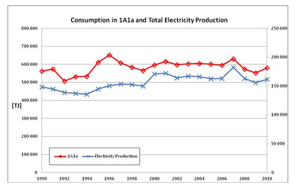
Fig. 3‑3 Correlation of 1A1a and Electricity production

In the final energy balance of CzSO (CzSO, 2011), the consumption of the individual kinds of fuels in this sector is reported in section Transformation Sector under the items:

· Main Activity Producer Electricity Plants

· Main Activity Producer CHP Plants

· Main Activity Producer Heat Plants

In the previous submissions autoproducers were also included in this category. This was discovered as a methodological mistake and this inaccuracy was corrected in current submission together with recalculation of 1A2 category. Detailed descriptions please see in relevant chapter for recalculation.

The category includes consumption of all kinds of fuels in enterprises covered by the NACE Rev. 2:

· 35.11 Production of electricity

· 35.30 Steam and air conditioning supply (production, collection and distribution of steam and hot water for heating, power and other purposes)

The following figure presents an overview of development of CO₂ emissions in source category 1A1a:

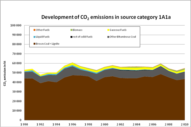
Fig. 3‑4 Development of CO₂ emissions in 1A1a category

Overall emissions show more or less stagnate trend with only a few oscillations. The decrease at the end of period is probably caused by reallocation of autoproducers to category 1A2.

The trend in emissions is mainly shaped by the development and structures of the electricity generation installations involved, since these installations account for the majority of the pertinent emissions. As is clear from the figure, solid fuels are the main driving forces for emissions in this source category. Brown Coal + Lignite are most important, with average consumption of 452 PJ, corresponding to 44 357 kt CO₂/year on an average for the whole 1990 – 2010 period. The second largest consumption is indicated for Other Bituminous Coal with an average consumption value of 78 PJ, corresponding to 7 169 kt CO₂/year on an average for the whole 1990 – 2010 period. The remaining solid fuels do not correspond to any significant consumption in this category.

Since 2007, the country-specific emission factor has been equal to 27.27 t C/TJ for Brown Coal + Lignite; a country-specific emission factor equal to 25.43 t C/TJ for Other Bituminous Coal and Coking Coal has been used to calculate CO₂ emissions. As mentioned above, this means that approximately 95% of the emissions from fuels in this category were determined using country-specific emission factors, i.e. at the level of Tier III.

Liquid fuels play a minor role in the electricity supply of the Czech Republic. They are used for auxiliary and supplementary firing in power stations – for instance stabilization of burners. Use of liquid fuels has decreased by more than half since 1990.

Natural Gas also plays a role in this source category. Use of NG does not exhibit a substantially changing trend. At the beginning of the period, it shows increasing trend, but later only minor changes were observed, which can be considered insignificant.

The item Other Fuels in Figure 3.4 represents waste consumption for waste incineration.

A specific question about the coal gasification facility was raised during the 2011 in-country review in Prague. The coal gasification facility originally produced town gas that was intended for distribution through the gas distribution system. Until 1995, consumption of this town gas was reported in different subsectors (1A1, 1A2 and 1A4) according to the purpose of use. In 1996, production of this town gas for the gas distribution system was stopped (it was completely replaced by natural gas). At the same time, the pressure gasification facility was reconstructed to a steam-gas cycle. Since 1996, the gas produced by pressure gasification (energy gas) is combusted in gas turbines for production of electricity and heat. Consequently, its consumption is reported under category 1A1a. The team is convinced that this reporting is in agreement with the methodology.

Other Fuels: Waste Incineration for energy purposes (1A1a)

This category consists of emissions caused by incineration of municipal solid waste for energy purposes. Originally this chapter was part of 6 C waste incineration but, based on the suggestion of ICR (in-country review), this chapter was shifted under the energy sector. This chapter is still prepared by CUEC (Charles University Environment Center) – the organization responsible for the waste sector.

This category consists of emissions of CO₂ from incinerated fossil carbon in MSW and emissions of methane and N₂O from incineration of MSW.

There are three municipal solid waste (MSW) incineration plants in the Czech Republic. One is located in Prague (ZEVO Malesice), one in Brno (SAKO) and the newest one in Liberec (Termizo). The incinerator in Brno was recently reconstructed (previous reporting year) and its former annual capacity of 240 Gg of MSW was decreased to 224 Gg of MSW. In actual fact, the new technology actually allowed the facility to be used to the full potential (the old stokers were regularly out of order and the real former capacity of the plant was about one third of the maximum value).

Tab. 3‑9 Capacity of municipal waste incineration plants in the Czech Republic, 2010

Incinerator	Capacity (Gg)
TERMIZO	96
Pražské služby a.s.	310
SAKO a.s.	224

There are also 76 other facilities incinerating or co-incinerating industrial and hazardous waste, with a total capacity 600 Gg of waste. This waste is reported under 6C.

All the parameters and calculations are shown in the following Tab. 3‑12

Tab. 3‑10 Parameters and emissions from waste incineration 1990-2010

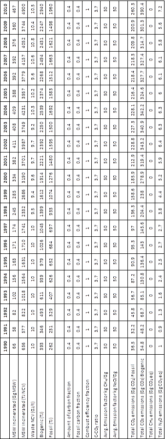
3.3.1.2 1A1b Petroleum refining

This category includes all facilities that process raw petroleum imported into this country as their primary raw material. Domestic petroleum constitutes approximately 3.5 % of the total amount. All fuels used in the internal refinery processes, internal consumption (reported by companies as “own use”) for production of electricity and heat and heat supplied to the public mains are included in emission calculations in this subcategory. This corresponds primarily to the Česká rafinérská, a.s. company in the Czech Republic. Fugitive CH₄ emissions are included in category 1B2Fugitive Emissions from Fuels - Oil.

The fraction of CO₂ emissions in subsector 1A1c in CO₂ emissions in sector 1A1 equalled 2 % in 2010. It contributed 1 % to CO₂ emissions in the whole ENERGY sector.

In the CzSO Questionnaire (CzSO, 2011), the consumption of the individual kinds of fuels in this sector is reported under the item:

· Refinery Fuel

· Relevant NACE Rev. 2 code: 19.20 - Manufacture of refined petroleum products

Greenhouse gas emissions in this subcategory are calculated using the national default emission factors at the Tier II level – see Table 3.11 – 3.14 net caloric values (NCV), CO₂ emission factors and oxidation factors used in the Czech GHG inventory.

Figure 3.5 depicts the correlation of CO₂ emissions in category 1A1b and CO₂ emissions from Crude Oil in the Reference Approach. These two features should have same trend and this is visible in the figure. The same trend is apparent in both categories at the end of the period; there is a peak in 2008 and the same shape of the curves between 2004 and 2006. At the beginning of nineties there were a great many technical innovations provided in refineries. The older technological facilities from the previous period were reconstructed, resulting in a decrease of energy intensity. This decrease in the energy intensity is connected with lower consumption of fuels even when the amount of processed oil was increasing.

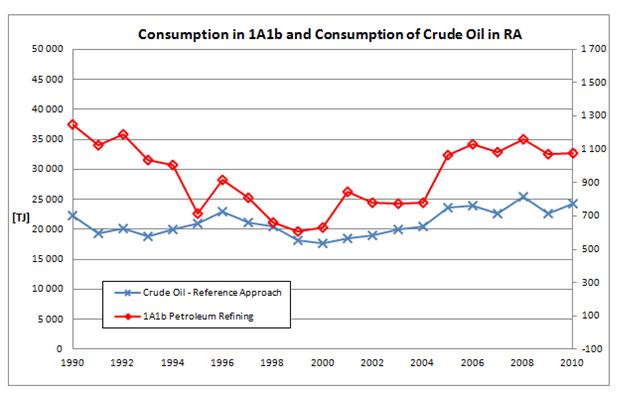
Fig. 3‑5 Correlation of CO₂ emission from 1A1b and from Crude Oil given in Reference Approach

The following figure shows an overview of emissions trends in source category 1A1b:

Fig. 3‑6 Development of CO₂ emissions in 1A1b category

It is apparent that no consumption of solid fuels occurred in this category.

Liquid fules are of the greatest importance and exhibit a decreasing trend at the beginnig and increasing trend at the end of the period. The fluctuations that have occurred over the years can be explained as resulting from differences in production quantities. The maximum production equal to 923 kt CO₂ occurred in 1990, followed by a value of 910 kt CO₂ in 2008. Thereafter, production decreased to the resulting level of 856 kt CO₂ in 2010.

The second greatest role is played by Natural Gas, with emissions in the range between 207 kt CO₂ in 2003 and 364 kt CO₂ in 1997 and resulting with 221 kt CO₂ in 2010.

3.3.1.3 1A1c Manufacture of solid fuels and other energy industries

This category includes all facilities that process solid fuels from mining through coking processes to the production of secondary fuels, such as Brown-Coal Briquettes, Coke Oven Gas or Producer Gas. It also includes fuels for the production of electrical energy and heat for internal consumption (reported by companies as “own use”).

There are a number of companies in the Czech Republic that belong in this category. These are mainly companies performing underground and surface mining of coal and its subsequent processing, located in the vicinity of coal deposits. The category also includes Coke plants and the production of Producer Gas. Other energy industries, such as facilities for extraction of Natural Gas and Petroleum are of minor interest in the Czech Republic.

The fraction of CO₂ emissions in subsector 1A1b in CO₂ emissions in sector 1A1 equaled 2.31 % in 2010. It contributed only 1.18 % to CO₂ emissions in the whole ENERGY sector.

In the CzSO Questionnaire (CzSO, 2011), the consumption of the individual kinds of fuels in this sector is reported in capture Energy Sector under the items:

· Coal Mines

· Oil and Gas Extraction

· Coke Ovens (Energy)

· Gas Works (Energy)

· Patent Fuel Plants (Energy)

· BKB Plants (Energy)

· Non-specified (Energy)

There are embodied the fuels of economic part according to NACE Rev. 2

· 05.10 Mining of Hard Coal

· 05.20 Mining of Lignite

· 06.10 Extraction of Crude Oil

· 06.20 Extraction of Natural Gas

· 19.10 Manufacture of Coke oven products (operation of Coke ovens, production of Coke and Semi-Coke, production of Coke Oven Gas)

· 19.20 Manufacture of refined petroleum products (this class also includes: manufacture of Peat Briquettes, manufacture of Hard-coal and Lignite fuel Briquettes)

The following figure provides an overview of emission trends in source category 1A1c:

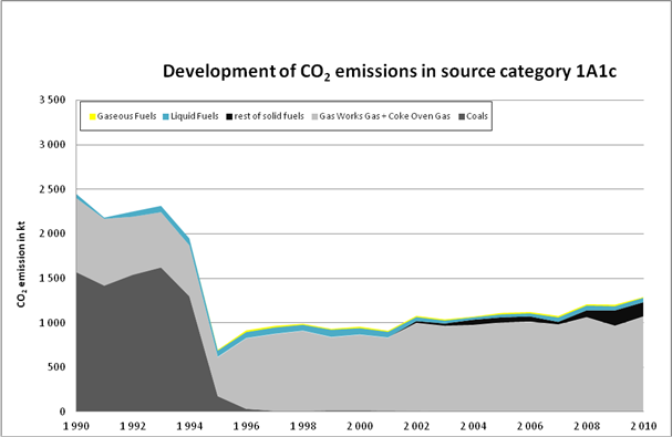
Fig. 3‑7 Development of CO₂ emissions in 1A1c category

The figure clearly shows a slow increase in emissions in 1995 – 2010 period. The use of coal predominated at the beginning of the period (i.e. Other Bituminous Coal, Brown Coal + Lignite and Coking Coal) and were later replaced by Gas Works Gas and Coke Oven Gas. There is very low use of liquid fuels and Natural Gas in this category.

Sokolovská Uhelná a.s makes the greatest contribution to the consumption of solid fuels . The section for processing Brown Coal was established in 1950 and also produced Gas Works Gas and other chemical products. Formally, the existence of this combine ended in 1974 when this facility was moved under the Hnědouhelné doly a briketárny company. Together with this step was established Fuel combine Vřesová. The new combined-cycle power station started to operate in 1996. This led to a sharp decrease in coal consumptions in 1994 – 1996 (http://www.suas.cz).

Coke Oven Gas is produced in the Ostrava area where are Coke Plants operating.

3.3.2 1A2 Manufacturing industries and construction

The fraction of CO₂ emissions in sector 1A2 in CO₂ emissions in the ENERGY sector equaled 22 % in 2010.

This source category consists of several sub-source categories defined in close harmony with the IPCC categorisations (CRF) and includes all stationary combustion emission sources that are not included in categories 1A1 and 1A4. It is described in detail via the relevant sub-chapters.

In previous submission the data for 1990 – 2002 period were reported as a sum for the entire sub-category group. Since 2003, the inventory has been performed in the detailed CRF structure. The originally used data from the national energy balance did not permit division of the fuel consumption into subsectors 1A2a to 1A2f and thus the data were reported for the entire category 1A2 Manufacturing industries and construction, in the CRF Reporter under subcategory 1A2f. This fact caused many question by ERTs and recommendations to disaggregate data and report them under relevant subcategories. Last recommendation was raised during the In country reviev in Prague in August/September 2011. Based on this recommendation it was prepared recalculation of this category and the data were disaggregated into relevant subcategories. Detailed explanations are given chapter for recalculation of this category.

Transition to the new format of source data (CzSO, 2011) permitted utilization of the data for more detailed classification in this subcategory.

· 1A2a Iron and steel

· 1A2b Non-ferrous metals

· 1A2c Chemicals

· 1A2d Pulp, paper and print

· 1A2e Food processing, beverages and tobacco

· 1A2f Other

The following figure shows developments in CO₂ emission trends in source category 1A2:

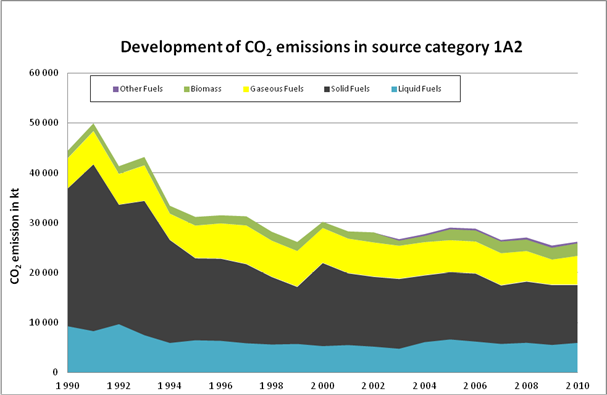
Fig. 3‑8 Development of CO₂ emissions in 1A2 category

It is clearly visible in the figure that solid fuels played the main role in emissions at the beginning of the period; however, the importance of solid fuels decreased over time. Currently, they are still of the greatest importance, but do not play such a dominant role in comparison with other fuels. Liquid Fuels indicate steady trend over the whole period – there is only a slight decrease at the beginning of the period. Natural Gas is also an important fuel in category 1A2.

3.3.2.1 1A2a Iron and steel

This category includes manufacturing in the area of pig iron (blast furnaces), rolling steel, casting iron, steel and alloys and is related only to ferrous metals. In the CzSO Questionnaire (CzSO, 2011), the consumption of the individual kinds of fuels in this sector is reported in capture Industry Sector under the item: Iron and Steel There are embodied the fuels of economic part according to NACE Rev. 2 Iron and steel: NACE Divisions 24.1 – 24.3 and 24.51, 24.52

Important facility belongs to this category is ArcelorMittal Ostrava, a.s. The fraction of CO₂ emissions in subsector 1A2a in CO₂ emissions in sector 1A2 equaled 15 % in 2010. It contributed only 3 % to CO₂ emissions in the whole ENERGY sector.

Fig. 3‑9. depicts the correlation of fuel consumption in category 1A2a Iron and Steel and production of pig iron (source: hz.cz). Obviously these two features should be correlated. A dissimilar trend is apparent at the beginning of the period, probably caused by inaccuracy in the activity data. In the next submission, we will exert an effort to improve these data. On the other hand, is apparent that the curve has the same shape in 1999, indicating good correlation.

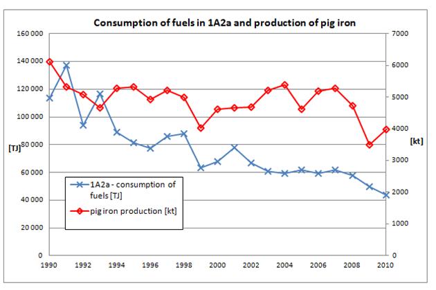
Fig. 3‑9 Correlation of fuel consumption in 1A2a with production of pig iron

3.3.2.2 1A2b Non-ferrous metals

This category encompasses combustion processes in various areas of production of nonferrous metals.In the Czech Republic, this corresponds mainly to foundry processes; primary production of nonferrous metals is not performed on an industrial scale in this country. In the CzSO Questionnaire (CzSO, 2011), the consumption of the individual kinds of fuels in this sector is reported in capture Industry Sector under the item:

· Non-Ferrous Metals

· There are embodied the fuels of economic part according to NACE Rev. 2

· Non-ferrous metals: NACE Divisions 24.4 , 24.53, 24.54

Important facility belongs to this category is Kovohutě Příbram. The fraction of CO₂ emissions in subsector 1A2b in CO₂ emissions in sector 1A2 equaled 0.5 % in 2010. It contributed only 0.1 % to CO₂ emissions in the whole ENERGY sector.

3.3.2.3 1A2c Chemicals

This subcategory includes all the processes in the organic and inorganic chemical industry and all related processes, incl. petrochemistry.

In the CzSO Questionnaire (CzSO, 2011), the consumption of the individual kinds of fuels in this sector is reported in capture Industry Sector under the item:

· Chemical (including Petrochemical)

· There are embodied the fuels of economic part according to NACE Rev. 2

· Chemicals: NACE Division 20

The fraction of CO₂ emissions in subsector 1A2c in CO₂ emissions in sector 1A2 equaled 50 % in 2010. It contributed 11 % to CO₂ emissions in the whole ENERGY sector.

Figure 3.10. depicts the correlation of fuel consumption in category 1A2c Chemicals and production of chemicals – source DEVELOPMENT OF OVERALL AND SPECIFIC CONSUMPTION OF FUELS AND ENERGY IN RELATION TO PRODUCT provided by CzSO. These two features should be correlated. There are also some dissimilarities in the trends, which we will try to correct in future submissions. The figure shows good agreement of both features after 2002.

Fig. 3‑10 Correlation of fuel consumption in 1A2c with production of chemicals

3.3.2.4 1A2d Pulp, paper and print

This subcategory includes all manufacturing processes related to the production of paper, cardboard and in printing plants. There are two primary paper production factories in the Czech Republic with a high consumption of waste wood from production processes. The other plants select the kind of fuel on the basis of the same criteria as the rest of the processing industry.

In the CzSO Questionnaire (CzSO, 2011), the consumption of the individual kinds of fuels in this sector is reported in capture Industry Sector under the item:

· Paper, Pulp and Printing

· There are embodied the fuels of economic part according to NACE Rev. 2

· Pulp, paper and print: NACE Divisions 17 and 18

The fraction of CO₂ emissions in subsector 1A2d in CO₂ emissions in sector 1A2 equaled 4 % in 2010. It contributed 1 % to CO₂ emissions in the whole ENERGY sector.

3.3.2.5 1A2e Food processing, beverages and tobacco

This subcategory includes all manufacturing processes related to the production of foodstuffs, beverages and foodstuff preparations. The subcategory also includes fuel consumption in the tobacco industry. The nature of the production processes permits the use of a relatively high fraction of biofuels.

In the CzSO Questionnaire (CzSO, 2011), the consumption of the individual kinds of fuels in this sector is reported in capture Industry Sector under the item:

· Food, Beverages and Tobacco

· There are embodied the fuels of economic part according to NACE Rev. 2

· Food processing, beverages and tobacco: NACE Divisions 10, 11 and 12

The fraction of CO₂ emissions in subsector 1A2e in CO₂ emissions in sector 1A2 equaled 5 % in 2010. It contributed 1 % to CO₂ emissions in the whole ENERGY sector.

Fig. 3‑11 depicts correlation of fuel consumption in category 1A2e Food processing, beverages and tobacco and production of food and beverages - source DEVELOPMENT OF OVERALL AND SPECIFIC CONSUMPTION OF FUELS AND ENERGY IN RELATION TO PRODUCT provided by CzSO. These two quantities apparently exhibit similar development over the whole time series.

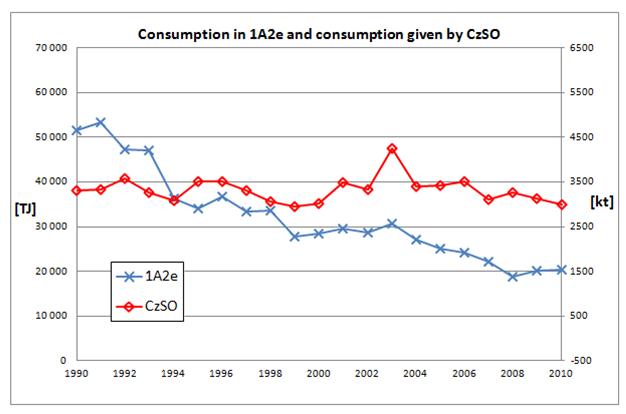
Fig. 3‑11 Correlation of fuel consumption in 1A2e with production of food and beverages

3.3.2.6 1A2f Other

This subcategory includes the remaining enterprises in the processing industry not included in subcategories 1A2a to 1A2e. This is an energy-demanding branch with high fuel consumption, such as the cement industry, lime production, the glass industry, production of ceramic materials, the textile and leather industry, wood processing and subsequent production processes, the entire machine industry, incl. production of means of transport and the construction industry.

In the CzSO Questionnaire (CzSO, 2011), the consumption of the individual kinds of fuels in this sector is reported in capture Industry Sector under the item:

· Non-Metallic Minerals

· Transport Equipment

· Machinery

· Mining (excluding fuels) and Quarrying

· Wood and Wood Products

· Construction

· Textiles and Leather

· Non-specified (Industry)

There are embodied the fuels of economic part according to NACE Rev. 2 Other: NACE Divisions 05 – 09, 13 – 16, 21 – 23, 25 – 33 and 41 - 43

In this year’s submission, this subcategory also includes the combustion of other kinds of fuel (Other Fuels). Activity data and data on CO₂ production were taken from the national ETS system (ETS, 2011), while CH₄ and N₂O emissions were calculated using the default emission factors for solid and liquid fuels. The fraction of CO₂emissions in subsector 1A2f in CO₂ emissions in sector 1A2 equaled 26 % in 2009. It contributed 6 % to CO₂ emissions in the whole ENERGY sector. Overall emissions indicate decrease since 1990. Solid fuels had at the beginnig of the period big importance, which constantly decrease untill 2010. Liquid fuels also constatnly descrease since 1990. Natural Gas has also apparent importance in this category.

Fig. 3‑12 Correlation of fuel consumption in 1A2f with production of cement and lime shows the correlation of fuel consumption in category 1A2f with production of cement and lime - source DEVELOPMENT OF OVERALL AND SPECIFIC CONSUMPTION OF FUELS AND ENERGY IN RELATION TO PRODUCT provided by CzSO.

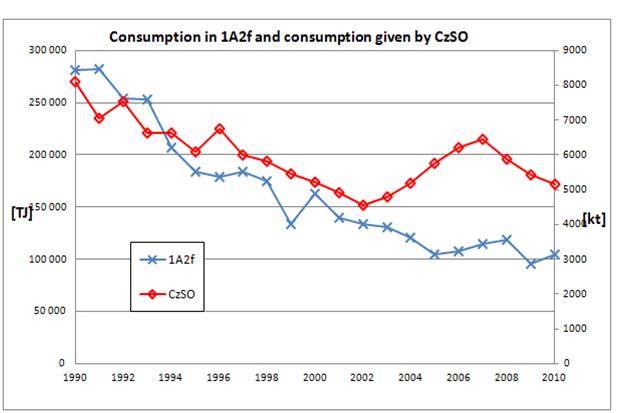
Fig. 3‑12 Correlation of fuel consumption in 1A2f with production of cement and lime

3.3.3 1A3 Mobile Combustion

Source category description

The categories of means of transport for the purposes of calculations of greenhouse gas emissions did not change compared to 2008. The criteria for inclusion of a certain means of transport in a particular category consist in the kind of transport, the fuel employed and the type of emission standard that the particular vehicle must meet (in road transport). The categories of vehicles are not as detailed for non-road transport.

The categories of mobile sources are following:

3.3.3.1 1A3a Civil Aviation

· airplanes fuelled by aviation gasoline

· airplanes fuelled by jet kerosene

3.3.3.2 1A3b Road transportation

· motorcycles,

· passenger and light duty gasoline vehicles conventional,

· passenger and light duty gasoline vehicles with EURO 1 limits,

· passenger and light duty gasoline vehicles with EURO 2 limits,

· passenger and light duty gasoline vehicles with EURO 3 limits,

· passenger and light duty gasoline vehicles with EURO 4 limits,

· passenger and light duty diesel vehicles conventional,

· passenger and light duty diesel vehicles with EURO 1 limits,

· passenger and light duty diesel vehicles with EURO 2 limits,

· passenger and light duty diesel vehicles with EURO 3 limits,

· passenger and light duty diesel vehicles with EURO 4 limits,

· passenger cars using LPG, CNG and biofuels (separately),

· heavy duty diesel vehicles and buses, conventional,

· heavy duty diesel vehicles and buses, with EURO 1 limits,

· heavy duty diesel vehicles and buses, with EURO 2 limits,

· heavy duty diesel vehicles and buses, with EURO 3 limits,

· heavy duty diesel vehicles and buses with EURO 4 limits,

· heavy duty diesel vehicles and buses using LPG, CNG and biofuels (separately).

3.3.3.3 1A3c Railways

· diesel locomotives

3.3.3.4 1A3d Navigation

· ships with diesel engines

3.3.3.5 1A3e Other transportation

The consumption of Natural Gas for powering compressors for the transit gas pipeline is included in this subcategory under mobile combustion sources, but in fact it is stationary combustion. This consumption is reported in the IEA – CzSO (CzSO, 2011) Questionnaire in the capture Transport Sector under the item:

· Pipeline Transport

There are embodied the fuels of economic part according to NACE Rev. 2 Pipeline Transport: NACE Divisions 35.22, 49.50

3.3.4 1A4 Other sectors

This category includes all the combustion processes in the sub categories described below. They can be generally defined as heat production processes for internal consumption.

The fraction of CO₂ emissions in sector 1A4 in CO₂ emissions in the ENERGY sector equaled 11 % in 2010.

The following figure depicts CO₂ emission trends in category 1A4:

Fig. 3‑13 Development of CO₂ emissions in 1A4 category

The main driving force for CO₂ emissions in category 1A4 is energy consumption for purposes of space heating. The fluctuations in consumption then can be ascribed to differences in cold winter periods. The trend of decreasing CO₂emissions is a result of higher standards for new buildings and of successful execution of energy-efficiency-oriented modernisations of existing buildings. The trend has also been supported by shifting to fuels with lower CO₂ emissions (emission factors).The importance of solid fuels at the beginning of the period, which constantly decreases in time, is apparent in the figure. On the other hand, the consumption of Natural Gas increased during the period as did Biomass consumption. Liquid fuels play a minor role in this category.

At the beginning of the period, a majority of households in the Czech Republic used coal as a heating fuel (mainly brown coal + lignite). This habit has changed over time and Natural Gas is beginning to be used more than solid fuels. The same trend appears in the institutional sphere. The number of households and institutions using biomass for heating (biomass boilers) in the Czech Republic has increased in the last few years. This trend is also apparent in the figure.

The winter of 2006 was colder than in other years, which also affected the consumption of fuels. Higher consumption of fuels for heating in households and institutions is apparent in this year. Significantly lower temperatures were recorded in the winter months in 2006 than in other years. The same trend is apparent in 2010.

3.3.4.1 1A4a Commercial/Institutional

This subcategory includes all combustion sources that utilize heat combustion for heating production halls and operational buildings in institutions, commercial facilities, services and trade.

In the CzSO Questionnaire (CzSO, 2011), the consumption of the individual kinds of fuels in this sector is reported in capture Industry Sector under the item:

· Commercial and Public Services

Where fuel consumption is reported here under the item:

· Non-specified (Other)

It is included under 1A4a Commercial/Institutional on the basis of an agreement with CzSO. There are embodied the fuels of economic part according to NACE Rev. 2 Commercial/Institutional : NACE Divisions 35 excluding 1A1a and 1A3e, 36 – 39, 45 – 99 excluding 1A3e and 1A5a

The fraction of CO₂ emissions in subsector 1A4a in CO₂ emissions in sector 1A4 equaled 31 % in 2010. It contributed 3 % to CO₂ emissions in the whole ENERGY sector.

3.3.4.2 1A4b Residential

Fuel consumption in households is determined on the basis of the results of the statistical study “Energy consumption in households”, published in 1997 and 2004 by the Czech Statistical Office according to the PHARE/EUROSTAT method.

In the CzSO Questionnaire (CzSO, 2011), the consumption of the individual kinds of fuels in this sector is reported in capture Industry Sector under the item:

· Residential

The fraction of CO₂ emissions in subsector 1A4b in CO₂ emissions in sector 1A4 equaled 67 % in 2009. It contributed 7 % to CO₂ emissions in the whole ENERGY sector.

3.3.4.3 1A4c Agriculture/Forestry/Fisheries

This subcategory contains combustion sources at stationary facilities for heating buildings, breeding and other operational facilities. The subcategory does not include fuel consumption for powering off-road means of transport and machinery. They are reported in category 1A5b Mobile - Agriculture, Forestry and Fishing.

In the CzSO Questionnaire (CzSO, 2011), the consumption of the individual kinds of fuels in this sector is reported in capture Industry Sector under the item:

· Agriculture/Forestry

· Fishing

There are embodied the fuels of economic part according to NACE Rev. 2 Agriculture/Forestry/Fisheries: NACE Divisions 01 - 03

The fraction of CO₂ emissions in subsector 1A4c in CO₂ emissions in sector 1A4 equaled 2 % in 2009. It contributed 0.21 % to CO₂ emissions in the whole ENERGY sector.

3.3.5 1A5 Other

The fraction of CO₂ emissions in sector 1A5 in CO₂ emissions in the ENERGY sector equaled 0.99 % in 2009.

3.3.5.1 1A5b Other – mobile sources

For reporting consumption of motor fuels, that was not report in sector 1A3 Transport and could not be reported in the other sectors as consumption of fuels in stationary sources is in CRF used this subcategory.

3.4 Methodological issues

3.4.1 Stationary combustion

The original data on the final national energy balance from CzSO (series of data in the 1990 – 1995 time series) were taken for the CRF structure directly in TJ. The time series from 1995 was constructed on the basis of data from the CzSO Questionnaire (CzSO, 2011), where the data on fuel consumption are given in various ways. Data are available for solid and liquid fuels in mass units (kt p.a.), where the net caloric values of these fuels are also tabulated. The consumption of gaseous fuels derived from fossil fuels is given in TJ p.a. Natural Gas is given in thousand m³ and the consumption in TJ is also tabulated; however, in this case it is calculated using the gross caloric value.

Consequently, the original calculation model was extended to include use of the net caloric value for processing data in the 1995 – 2010 time series. In 2011 we got from CzSO calorific values for liquid fuels for the whole time series and these are now assumed to be right (agreed by CzSO) and therefore used for conversion of activity data from natural units to energy units.

One recalculation was performed in this submission. The main reason for the recalculation was an attempt to extend data division into each subcategory in category 1A2 back to 1990. The data available in the CzSO Questionnaires for 1990 – 1994 are not sufficiently reliable for emission calculation; therefore, the recalculation was performed for the 1995 – 2009 period using the data from CzSO and, before 1995, the summary values which were originally in subcategory 1A2f Other were disaggregated into each subcategory according to the development of the relevant branch of industry and other indicators. It was also necessary to perform this recalculation for other source categories to ensure consistency of data use. Therefore, the recalculation was also performed in categories 1A1, 1A3e, 1A4, 1A5, 1AD using the activity data from the CzSO Questionnaires in the 1995 – 2009 period. For the 1990 – 1994 period, the original data on the final national energy balance calculated according to the CzSO methodology were used. Detailed descriptions of recalculations are given in chapter 3.7.1.

The principles of preparation of the emission inventory are further specified in detail for the individual phases of data preparation and processing and subsequent utilization of the results of calculations with subsequent storage.

Collection of activity data

In collection of activity data, all the background data are stored at the workplace of the sector compiler, where possible in electronic form. These consist primarily in datasets obtained from CzSO as officially submitted data for drawing up the activity data. The datasets are unambiguously designated and cited under this designation.

If the data are taken from the Internet, the relevant passages (texts, tables) are stored in separate files with designation of the web site where they were obtained and the date of acquisition.

Data taken from printed documents are suitably cited, the written documents are stored in printed form at the workplace of the sector compiler and, where possible, the relevant passages (texts, tables) are scanned and stored in electronic form.

When the stage is completed, all the stored data are transferred to electronic media (CD, external HD, flash disks, etc.) and stored with the sector compiler; the most important working files that contain data sources, calculation procedures and the final results are submitted in electronic form for storage at the coordination workplace.

Conversion of activity data to the CRF format

The activity data are converted from the energy balance to the CRF structure in the EXCEL format.

Each working file has a “Title page” as the first sheet.

The Title page shall contain particularly the following information:

· the name and description of the file

· the author of the file

· the date of creation of the file

· the dates of the latest up-dating, in order

· the source of the data employed

· description of transfer of specific data from the source files

· the means of aggregation of the data base employed in conversion

· explanations and comments.

The working files shall also contain a compulsory “Activity Data” Sheet. The Activity Data Sheet shall contain:

· complete division of the data into IPCC (SA) sectors and subsectors or individual fuels for

· RA, in structure compatible with CRF

· complete time series

the units in which the activity data balance is drawn up

The conversion shall be performed in two separate sets for the Sectoral Approach (SA) and Reference Approach (RA). If the data conversion requires recalculation from natural units to energy units, the calorific values of the individual kinds of fuels used is included in the calculation. The calorific values employed are stored.

Calculations of emissions

These values are given in the following sheets of the working files, which also contain the “Emission Factors” sheet, the “Oxidation Factors” sheet and calculation sheets for the individual GHG gases. The necessary aggregations for transfer of the data to the CRF reporter are included.

Original activity data are given in kilotons. It means that it is necessary to convert these values to energy units – terajoules. For this conversion are used calorific values. In 2011 it was new calorific values for liquid fuels agreed by CzSO and are therefore used for calculation of emissions. Comparison of old and new calorific values is given in table 3.12.

Tab. 3‑11 Net caloricic values used in the Czech GHG inventory – 2010

NCV [TJ/Gg]	1A1a	1A1b	1A1c	1A2	1A4a	1A4b	1A4c	1A5
NCV [TJ/Gg]	1A1a	1A1b	1A1c	1A2	1A4a	1A4b	1A4c	1A5
Refinery Gas		42.23
LPG				43.82	43.82	43.82	43.82
Naphtha				43.96
Gasoline						43.40		43.40
Kerosene Jet Fuel					43.30			43.30
Other kerosene				0.00	42.80
Diesel Oil			42.75	42.75				42.75
Heating and Other Gasoil	42.60		42.60	42.60	42.60		42.60
Fuel Oil - Low Sulphur	39.70	39.70		39.70	39.70		39.70
Fuel Oil - High Sulphur				39.49
Lubricants				40.19
Other Oil		39.82		39.82
Anthracite				30.00
Other Bituminous Coal	22.55			23.19	28.45	28.45	28.45
Brown Coal + Lignite	12.47		12.67	12.67	13.84	13.84	13.84
Coke				27.99	28,06	28,06	28,06
Coal Tars			36.94	36.94
Brown Coal Briquettes	23.00					20.74

Tab. 3‑12 Comparison of calorific values used in previous and current submission (part 1)

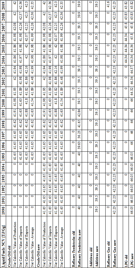
Tab. 3‑12 Comparison of calorific values used in previous and current submission (part 2)

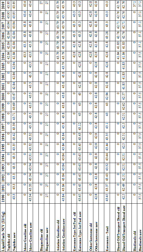
Tab. 3‑12 Comparison of calorific values used in previous and current submission (part 3)

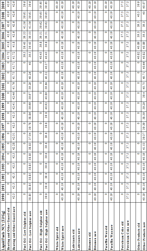
Tab. 3‑12 Comparison of calorific values used in previous and current submission (part 4)

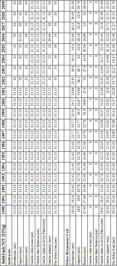
Tab. 3‑12 Comparison of calorific values used in previous and current submission (part 5)

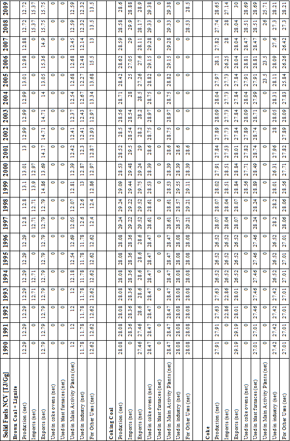
Tab. 3‑12 Comparison of calorific values used in previous and current submission (part 6)

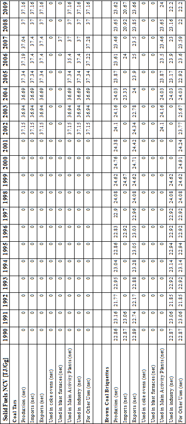
Coke Oven Gas, Gas Works Gas and biofuels in the CzSO Questionnaires are given directly in terajoules, so that calorific values are not used in these cases. The data for Coke Oven Gas and Gas Works Gas in TJ were calculated using the gross calorific values, so it is necessary to recalculate these values to net calorific values.

Natural Gas is given in the statistic reporting in the CzSO Questionnaire (CzSO, 2011) in thousand m3 and in TJ; however, the data in TJ was calculated using the gross caloric value.

Information on the average values of the gross caloric value and the net caloric value of Natural Gas are given in Tab. 3‑13.

Recalculation of volume units to mass units for Natural Gas was performed using the density 0.69 kg/m³ (t = 15 °C, p = 101.3 kPa).

Tab. 3‑13 Average values of the gross caloric value and the net caloric value of Natural Gas – Questionnaire IEA – CzSO (CzSO, 2011), 2010

[TJ/Gg]	GCV	NCV	GCV/NCV
Indigenous Production	38.32	34.49	1.11
Associated Gas	39.03	35.13	1.11
Non-Associated Gas	36.88	33.19	1.11
Total Imports (Balance)	38.14	34.32	1.11
Total Exports (Balance)	38.13	34.32	1.11
Stock Changes (National Territory)	38.20	34.38	1.11
Inland Consumption (Calculated)	38.15	34.33	1.11
Inland Consumption (Observed)	38.14	34.33	1.11
Opening Stock Level (National Territory)	38.25	34.43	1.11
Closing Stock Level (National Territory)	38.30	34.47	1.11

The values of consumption of Natural Gas were taken from this statistical report in TJ and the values were then divided by a coefficient of 1.11 for recalculation from the gross caloric value to the net caloric value.

The greenhouse gas emissions were calculated as the product of the activity data and the relevant emission factor. A survey of the emission factors employed for CO₂ is given in Table 3.14. The experimentally determined country-specific values of the emission factors were used for Coal and Lignite (Fott, 1999); for the other fuels, the default emission factors from the IPCC methodology (IPCC, 1997) were used. Oxidation factors used in the national inventory are the default values taken from the IPCC methodology (IPCC, 1997).

Tab. 3‑14 Net caloricic values (NCV), CO₂ emission factors and oxidation factors used in the Czech GHG inventory – 2010

Fuel (IPCC 1996 Guidelines	NCV	CO₂ EF ^a)	Oxidation	CO₂ EF ^b)
definitions)	[TJ/Gg]	[t CO₂/TJ]	factor ^e)	[t CO₂/TJ]
Crude Oil	42.4	73.33	0.99	72.59
Gas / Diesel Oil	42.75	74.10	0.99	73.35
Residual Fuel Oil	39.59	77.40	0.99	76.62
LPG	43.82	63.10	0.995	62.78
Naphtha	43.96	73.30	0.99	72.56
Bitumen	40.19	80.67	0.99	79.86
Lubricants	40.19	73.30	0.99	72.56
Petroleum Coke	37.50	97.5	0.98	95.55
Other Oil	39.82	73.30	0.99	72.56
Coking Coal ^d)	29.39	93.24	0.98	91.37
Other Bituminous Coal ^d)	23.19	93.24	0.98	91.37
Lignite (Brown Coal) ^d)	12.67	99.99	0.98	97.99
Brown Coal Briquettes	20.82	97.49	0.98	95.54
Coke Oven Coke	27.93	106.99	0.98	104.85
Coke Oven Gas (TJ/mill. m³)	15.62^c)	44.4	0.995	44.17
Natural Gas (TJ/Gg)	57.22	56.10	0.995	55.81
Natural Gas (TJ/mill. m³)	34.33^c)	56.10	0.995	55.81

a) Emission factor without oxidation factor

b) Resulting emission factor with oxidation factor

c) TJ/mill. m³, t= 15°C, p = 101.3 kPa

d) Country specific values of CO₂ EFs

e) Oxidation factors values used for national inventory of greenhouse gases are 0.995 for gaseous fuels, 0.99 for liquid fuels and 0.98 for solid fuels

Methane emissions from fuel combustion from stationary sources do not constitute key sources. Relatively the largest contribution comes from fuel combustion in local heating units.

The means of determining methane emissions is similar in many respects to the method of the individual consumption categories for carbon dioxide emissions. The simplest level (Tier 1) (IPCC, 1997) includes only summary fuel categories:

· coal-type solid fuels

· gaseous fuels

· liquid fuels

· wood fuel (biomass)

· other biomass.

Only the first four categories were filled with activity data in the inventory. These data were aggregated directly from the connected working sheets for the calculation of carbon dioxide by the consumption sector method.

Tab. 3‑15 CH₄ emission factors in the individual sectors used in the Czech GHG inventory (1990 – 2010)

[kg CH₄/TJ]	1A1	*1A2^)**	1A3e	1A4a	1A4b	1A4c
Liquid fuels	3	2		10	10	10
Solid fuels	1	10		10	300	300
Gaseous fuels	1	5	5	5	5	5
Biomass	30	30		300	300	300

*) The emission factors are also valid for the other kinds of fuels (Other Fuels).

N₂O emissions from stationary sources do not belong amongst key sources in the CR.

In 2008 N₂O emissions from combustion of all kinds of fuel were recalculated using the default emission factors over the entire time series.

This submission employed the emission factors for N₂O in all the sectors as tabulated below (uniformly for the entire sector of stationary combustion sources):

Liquid fuels	0.6 kg N₂O/TJ
Solid fuels	1.4 kg N₂O/TJ
Gaseous fuels	0.1 kg N₂O/TJ
Biomass	4.0 kg N₂O/TJ

A considerable part of the non-energy consumption consists in non-energy consumption of petroleum (lubricating and special oils, asphalt and particular petrochemical raw materials used for the production of plastic materials, etc.). Non-energy products formed from Bituminous Coal in Coke plants and from Brown Coal in the production of coal gas (historical) and energy gas (fuel for the combined steam-gas cycle) are also important.

In this context, emphasis is placed on the correct determination of the fraction of stored (fixed) carbon in the non-energy use of fossil fuels. Calculation of its amount is based on the assumption that a certain amount of the carbon contained non-energy raw materials remains fixed in the long term and is not released as CO₂. In the energy balance CzSO (CzSO, 2010), this consists in:

petrochemical raw materials (Naphtha) mainly used for the production of plastic materials
lubricating oils (Lubricants)
Coal Tars from coking of Bituminous Coal and from gasification of Brown Coal
asphalt (Bitumen)

Part of the intermediate products from pyrolysis of petrochemical raw materials is used directly as heating gases and oils, part of the final products (plastic materials) are also burned after use in municipal waste incinerators, but part ends up in land-fills. Thus, a considerable part of the input carbon remains bonded for a longer time in plastic materials. As plastic materials are being increasingly recycled, the fraction of carbon stored in plastics has been gradually increased from 50% to 80% between 2003 and 2006 (in period 1990 - 2002 this fraction was considered constant, 50%).

In addition, most lubricating and special oils are finally used as heating oils or are burned during their use (lubricating oils for combustion motors). Part of the oils is used for production of alternative fuels and part is burned in incinerators, but at least half remains permanently anchored in lubricants.

Consequently, a fraction of stored carbon of 50% is used in the balance.

Coal tars have a similar fate and are also used for impregnation of roofing materials and for soot (additive in the production of rubber). Consequently, a value of stored carbon fraction of 75 % is used.

Practically one hundred percent fixation is assumed for asphalt.

Data on the consumption of other fuels are newly used in the greenhouse gas inventories. Information on the consumption of Other Fuels was taken from the national ETS database (ETS, 2009) and is related only to the use of these fuels in cement production.

In the submission 2009, the data on consumption of Other Fuels was processed for the first time and the time series from 2003 to 2008 was drawn up. Data were employed as provided by the Federation of Cement Producers of the Czech Republic (Federation of Cement Producers of the Czech Republic, 2009). The database contains detailed information on consumption of the individual kinds of alternative fuels, their calorific values and emission factors. The same data source was also employed for processing data for 2010 (Federation of Cement Producers of the Czech Republic, 2011). The default emission factors were employed for calculation of the CH₄ and N₂O emissions according to the character of the relevant fuel.

Tab. 3‑16 Consumption and EF – Other fuels in the cement industry in 2010

Kind of	Consumption	EF
Fuel	[TJ/year]	[t CO₂/TJ]	[kg CH₄/TJ]	[kg N₂O/TJ]
Solid	3224.48	83.52	10	1.4
Liquid	707.57	80.40	2	0.6

Tab. 3‑17 CO₂, CH₄ and N₂O Emissions from use of Other fuels in the cement industry in 2010

Kind of	Emission [kt/year]
Fuel	CO₂	CH₄	N₂O
Solid	269.3	0.0322	0.00451
Liquid	56.9	0.0014	0.00042
Total	326.2	0.0337	0.00494

Other Fuels (1A1a)

This category follows Tier 1 methodology for emissions from waste incineration. Consistent with the 1996 Guidelines (IPCC, 1997), only CO₂ emissions resulting from oxidation, during incineration and open burning of carbon in waste of fossil origin (e.g., plastics, certain textiles, rubber, liquid solvents, and waste oil) are considered in the net emissions and should be included in the national CO₂ emissions estimate.

Estimation of CO₂ emissions from waste incineration is based on the Tier 1 approach (Good Practice Guidance, 2000). It assumes that total fossil carbon dioxide emissions are dependent on the amount of carbon in waste, on the fraction of fossil carbon and on the combustion efficiency of the waste incineration. As no country-specific data were available for the necessary parameters, the default data for the calculation were taken from the IPCC Good Practice Guidance. All parameters and calculations are shown in the Table 3.10.

1A3e Other transportation

An emission factor of 15.3 t C/TJ was used for the estimate.

According to the ERT recommendation of 2009, default emission factors are used for CH₄ and N₂O in the entire time series.

3.4.2 1A3 - Mobile Combustion

Important information about the International Bunkers category and its subcategories was verified in 2010. On the recommendation of ERT, the subcategories Aviation Gasoline and Marine Diesel Oil in International Bunkers were verified. No more information about fuel consumption, passenger transport or transport of goods is available in any of these categories (MTC, 2000; MTC, 2006; MTC, 2011) in the Czech Republic. Based on this fact, notation keys “NO” in the Marine category were retained and notation keys in the Aviation Gasoline category were changed from “NE” to “NO”. The important problem with inconsistent data on fuel consumption of Jet Kerosene in Aviation (Domestic and International) was solved and described in Chapter 3.7.2. (recommended by ERT).

CO₂ emissions

Carbon dioxide emissions were calculated on the basis of the total consumption of the individual automotive fuels used in transport (i.e. gasoline, diesel oil, LPG, CNG, biofuels and aviation fuels) and the emission factors for the weight of CO₂ corresponding to 1 kg of fuel burned. Consumption of the individual kinds of fuel by road, railway and water transport was determined on the basis of cooperation with the CzSO. Consumption in road transport was further divided up into the following categories of means of transport on the basis of statistics on transport output:

· gasoline-fuelled passenger vehicles;

· diesel vehicles for passenger and light freight transport;

· diesel vehicles for heavy freight transport and buses;

· passenger and light vehicles fuelled by LPG, CNG and biofuels (separately);

· heavy trucks and buses fuelled by LPG, CNG and biofuels (separately).

The share of transport in total CO₂ emissions has exhibited an increasing trend in the Czech Republic during the 90’s and this growth is continuing until 2007. Individual road and freight transport make the greatest contribution to energy consumption in transport. The amount of fuel sold is monitored annually and constitutes the main input data for calculation of energy consumption.

In 2008, for the first time, emissions of carbon dioxide from transport exhibited a decrease, which started a downward trend continuing until 2010 (Jedlicka et al, 2009). The reduction in carbon dioxide emissions was a result primarily of a reduction in the consumption of gasoline and diesel oil, which is interpreted as being a consequence of the global economic crisis. The downward trend in fuel consumption is evaluated very favourably from viewpoint of greenhouse gases.

There was a decrease in fuel consumption in 2010, continuing the downward trend of 2009. However, this persistent downward trend may no longer be a consequence of the economic crisis. This phenomenon may be caused by the cross-border purchases of gasoline and especially diesel fuel. The price of diesel fuel in the Czech Republic is much higher than in neighbouring countries and is one of the highest in Europe. The increase in fuel prices is related to the excise tax imposed by the Czech legislation. The greenhouse gas emission balance reflects not only the scenario of consumption of alternative fuels, but also the scenario of trends in the transport infrastructure, further construction of the throughway network in different variants, urban bypasses, further construction of railway corridors, etc.

The consumption of gasoline has fluctuated around 2 million tonnes since 2002. Since 2008, the consumption of gasoline also has included the consumption of bioethanol, which has been added to all gasoline in an amount of 2 % since January 1, 2008. The fraction of bioethanol as a renewable resource in gasoline reached a value 4.1 % in 2010 and will continue to increase in the coming years. Thus the actual consumption of gasoline without inclusion of biofuels is less by the percentage of bioethanol. These facts (reduction in consumption and increasing the share of bio-components) have a favourable impact on CO₂ emissions.

Mobile sources used for purposes other than transport – gasoline-powered lawn mowers, chain saws, construction machinery, etc. – make a smaller contribution to the increasing consumption of gasoline and diesel oil.

In relation to CO₂ emissions from air transport, it can be stated that domestic transport makes a very small contribution to these emissions – about 1 %, as it is limited mainly to flights between the three largest cities in the Czech Republic, Prague, Brno and Ostrava. Similar to road transport and consumption of aircraft fuel, this is not monitored centrally by the Czech Statistical Office. Aircraft are fuelled mainly by jet kerosene, while the consumption of and CO₂ emissions from aviation gasoline are limited to small aircraft used in agriculture and in sports and recreational activities.

The total consumption of the army and the consumption of the domestic transport (estimated on the basis of the number of flights, distances between destinations and the specific consumption of fuels per the unit of distance in the LTO regime and the cruise itself) were subtracted from the total kerosene consumption. The remaining kerosene consumption is related to the international air transport.

Carbon dioxide emissions for the 2000 – 2006 time series were recalculated in 2008. The reasons for the recalculation and more detailed information are given in the Chapter 10.1.3.

Tab. 3‑18 CO₂ emissions calculation from mobile sources in 1990 – 2010 [Gg CO₂]

	Aviation (without Bunkers)	Road Transportation	Railways	Navigation	Other Transport Pipeline transport	Other Mobile Agric. and others	Total
	1.A3a	1.A3b	1.A3c	1.A3d	1.A3e	1.A5b	1.A3 + 1.A5
1990	145.9	6 239	651.5	56.4	494.4	1 601	9 188
1991	40	5 616	580.2	56	501.5	1 409	8 203
1992	40.7	6 494	492.4	54.6	547.4	1 321	8 950
1993	24.8	6 610	413.6	54.1	442.6	1 276	8 821
1994	22.9	7 147	333.4	53.3	312.5	1 285	9 154
1995	14	9 180	332.7	55	36.5	1 191	10 809
1996	15.9	10 227	328	45.8	88.8	1 141	11 847
1997	10.4	10 997	282.1	38.4	76.2	1 189	12 593
1998	10.2	11 167	354.6	37.7	58.9	1 264	12 892
1999	13.2	11 391	329.5	22	63.0	1 245	13 064
2000	11.3	11 521	326.4	15.7	58.8	1 235	13 168
2001	8.2	12 375	304.4	25.1	60.1	1 194	13 967
2002	11.1	12 966	295	12.6	62.3	1 140	14 487
2003	11.4	14 759	288.7	12.6	58.9	1 061	16 192
2004	12.3	15 520	285.6	18.8	56.8	1 107	17 000
2005	9.2	16 840	288.7	15.7	69.4	1 094	18 317
2006	9.8	17 146	301.2	18.8	74.3	1 074	18 624
2007	9.8	18 029	298.1	15.7	120.2	1 085	19 558
2008	8.6	17 826	329.5	12.6	147.6	1 133	19 457
2009	8	17 290	298.1	15.7	153.1	1 117	18 882
2010	9.1	16 268	288.7	12.6	152.8	1083	17 814

CH₄ emissions

For road transportation, the method of methane emission calculation corresponds to the Tier 2 level, because different road vehicles produce different amounts of methane. It can be stated that methane emissions from road transportation exhibit the same differences as total hydrocarbons. Mobile emission sources were divided up into several categories according to the fuel used, the transport mode and the emission limit that a particular vehicle must meet. This division is more detailed because there are larger differences in methane production by individual vehicles. These categories are described in detail in Chapter 3.3.1 "Source category description".

The total consumption of gasoline, diesel oil, LPG, CNG and biofuels has been determined from the statistical surveys of the CzSO. The next step consisted in separation of these fuel consumptions into the vehicle categories described above, according to their transport outputs acquired in the last National Traffic Census performed in the Czech Republic once every five years, last in 2005. The emission factors were the IPCC default values and, from 2004, the country-specific values as CDV became part of the emission inventory team.

The Czech Republic has been very successful in stabilizing and decreasing methane emissions derived from transport-related greenhouse gas emissions. The annual trends in these emissions are constantly decreasing and are very similar to other hydrocarbons emissions, which are limited in accordance with UN ECE regulations. New vehicles must fulfill substantially higher EURO standards for hydrocarbons than older vehicles (currently the EURO IV standard). The greatest problems are associated with the slow renewal of the freight transport fleet. There has been almost no decrease in the number of older trucks in this country and these older vehicles are frequently used in the construction and food industries (Adamec et al, 2005a).

Methane emissions from mobile sources are now calculated using methane emission factors taken from the internal database, containing both data from Czech emission measurements (mostly obtained from the Motor Vehicle Research Institute - TÜV UVMV) and internationally accepted values from the IPCC methodology, European Environmental Agency - Emission Inventory Guidebook, CORINAIR, etc. The resultant emission factors were calculated using the weighted averages of all data classified according to transport vehicle categories. The following categories were included: conventional gasoline-fuelled passenger cars, gasoline-fuelled passenger cars fulfilling EURO limits, diesel-fuelled passenger cars, light-duty vehicles, heavy-duty vehicles, diesel locomotives, diesel-fuelled watercraft, aircraft fuelled by aviation gasoline and kerosene-fuelled aircraft (Adamec et al, 2005b).

Emissions of CH₄ from mobile sources are given in Table 3.15 CH₄ emissions calculation from mobile sources in 1990 – 2010 [Mg CH₄]

Tab. 3‑19 CH₄ emissions calculation from mobile sources in 1990 – 2010 [Mg CH₄]

	Aviation (without Bunkers)	Road Transportation	Railways	Navigation	Other Transport Pipeline transport	Other Mobile Agric. and others	Total
	1.A3a	1.A3b	1.A3c	1.A3d	1.A3e	1.A5b	1.A3 + 1.A5
1990	28.58	1 260	40.86	3.54	44.29	335.7	1 712.98
1991	7.8	1 098	36.39	3.51	44.92	291.9	1 482.55
1992	7.92	1 318	30.89	3.43	49.04	270.1	1 679.33
1993	4.79	1 336	25.95	3.39	39.65	262.0	1 671.79
1994	4.38	1 449	20.91	3.34	28.00	264.0	1 769.58
1995	2.71	1 638	20.87	3.45	3.27	242.8	1 911.08
1996	3.2	1 798	20.57	2.87	7.96	221.0	2 053.61
1997	1.92	1 883	17.69	2.41	6.83	191.0	2 102.86
1998	1.88	1 851	22.24	2.36	5.28	144.7	2 027.48
1999	2.48	1 839	20.67	1.38	5.65	98.6	1 967.75
2000	2.16	1 716	20.47	0.98	5.27	84.6	1 829.47
2001	1.55	1 739	19.9	1.57	5.38	82.0	1 849.37
2002	2.13	1 630	18.5	0.79	5.58	81.3	1 738.33
2003	2.18	1 681	18.11	0.79	5.27	74.1	1 781.43
2004	2.32	1 598	17.91	1.18	5.09	78.3	1 702.81
2005	1.72	1 610	18.11	0.98	6.22	77.9	1 714.94
2006	1.82	1 517	18.9	1.18	6.65	75.0	1 620.56
2007	1.82	1 517	18.7	0.98	10.77	78.3	1 627.53
2008	1.61	1 462	20.67	0.79	13.22	81.4	1 579.65
2009	1.52	1 393	18.7	0.98	13.72	81.2	1 509.10
2010	1.7	1 224	18.11	0.79	13.68	76.4	1 334.71

N₂O emissions

Nitrous oxide emissions decreased in 2008 similar to carbon dioxide emissions as a consequence of reduced consumption of gasoline and diesel oil. Newer vehicles exhibit higher emissions compared to older models, because they are equipped with 3-way catalytic converters, which reduce only NO_x emissions but not N₂O emissions. However, this effect is suppressed in the new vehicles as a consequence of production of vehicles with lower fuel consumption. Between 2008 and 2010, the downward trend in N₂O emissions still continued in a similar to carbon dioxide emissions.

Road transport was identified as a key source of N₂O emissions over the past 4 years, as the share of vehicles with high N₂O emissions has been increasing over this time. Consequently, N₂O emissions from mobile sources represent a somewhat more important contribution than CH₄ emissions. In calculation of N₂O emissions from mobile sources, the most important source according to the IPCC methodology seems to be passenger automobile transport, especially gasoline-fuelled passenger cars with catalysts. The vehicle categories for the nitrous oxide calculation are the same as for methane (see above).

Because of big differences between national N₂O measurement results and values recommended in IPCC methodology, the special verification including the statistical evaluation has been performed. The resulted values of N₂O emission factors from mobile sources are approaching to recommended IPCC values. The emissions factors for N₂O for vehicles with diesel motors and for vehicles with gasoline motors without catalysts are not very high and were taken in the standard manner from the methodical instructions (IPCC default values). The situation is more complex for vehicles with gasoline motors equipped with three-way catalysts. The IPCC methodology (IPCC, 1997) gives three pairs of emission factors for passenger cars with catalysts (for new and deactivated catalysts). The value for a deactivated catalyst is approximately three times that for a new catalyst. The pair of values recommended on the basis of Canadian research was selected because of the lack of domestic data; in addition, American and French coefficients are presented in the IPCC Reference Manual, Box 3 (IPCC, 1997). The arithmetic mean of the values for new and older used catalysts was taken as the final emission factor for passenger cars with catalysts.

A partial increase in N₂O emissions can be expected in this category in connection with the growing fraction of vehicles equipped with three-way catalysts. This approach described above was recently revised and modified by CDV, which is a member of the Czech national GHG inventory team from 2005. CDV has been providing the transport data for the official Czech inventory since 2004. The CDV approach is based on combination of measurements performed for some cars typically used in the Czech Republic with widely used EFs values taken from literature (Dufek, 2005).

The situation in relation to reporting N₂O emissions is rather complicated, as some of the measurements performed in the past in the Czech Republic were substantially different from the internationally recognized emission factors. Consequently, control measurements were performed on N₂O emissions from the commonest cars in the Czech passenger vehicle fleet (Skoda Felicia, Fabia and Octavia) during 2004 - 2006 years. These corrections brought the results closer to those obtained using IPPC emission factors than the older data, leading to better harmonization of the results of the nitrous oxide emission inventory per energy unit with those obtained in other countries. The locally measured data for measurements of N₂O emissions in exhaust gases were verified by assigning weighting criteria for each measurement; the most important of these criteria were the number of measurements, the analysis method, the type of vehicle and the fraction of these vehicles in the Czech vehicle fleet. (Dufek, 2005 and Jedlicka et al, 2005).

Nitrous oxide emission factors were obtained using a similar method to that employed for methane, by statistical evaluation of the weighted averages of the emission factors for each category of vehicle (see Chapter 3.1.3), employing the interactive database. This database now encompasses the results of the Czech measurements performed in 2004 and 2005 (Adamec et al, 2005b). Emissions of N₂O are given in Tab. 3‑20 N₂O emissions calculation from mobile sources in 1990 – 2010 [Mg N₂O].

Tab. 3‑20 N₂O emissions calculation from mobile sources in 1990 – 2010 [Mg N₂O]

	Aviation (without Bunkers)	Road Transportation	Railways	Navigation	Other Transport Pipeline transport	Other Mobile Agric. and others	Total
	1.A3a	1.A3b	1.A3c	1.A3d	1.A3e	1.A5b	1.A3 + 1.A5
1990	20.19	425	37.37	3.24	0.89	63.2	549.89
1991	5.53	377.5	33.28	3.21	0.90	55.0	475.45
1992	5.63	479.9	28.25	3.13	0.98	51.1	568.99
1993	3.43	522.9	23.73	3.1	0.79	50.0	603.96
1994	3.17	610.3	19.12	3.6	0.56	49.7	686.44
1995	1.93	759.1	19.9	3.16	0.07	46.3	830.49
1996	2.19	875.5	18.81	2.63	0.16	44.9	944.17
1997	1.44	954.4	16.18	2.2	0.14	53.7	1028.02
1998	1.41	1049.8	20.34	2.16	0.11	75.6	1149.38
1999	1.83	1161.9	18.9	1.26	0.11	81.0	1265.05
2000	1.56	1255.5	18.72	0.9	0.11	82.6	1359.41
2001	1.14	1408.5	17.46	1.44	0.11	80.0	1508.63
2002	1.53	1588.5	16.92	0.72	0.11	78.2	1685.93
2003	1.58	1893.1	16.56	0.72	0.11	71.8	1983.85
2004	1.7	2059.6	16.38	1.8	0.10	75.5	2155.07
2005	1.27	2203.4	16.56	0.9	0.12	74.9	2297.17
2006	1.36	2234.8	17.28	1.8	0.13	72.7	2328.06
2007	1.36	2338.1	17.1	0.9	0.22	74.9	2432.54
2008	1.18	2299.7	18.9	0.72	0.26	78.0	2398.73
2009	1.1	2258.9	17.1	0.9	0.27	77.4	2355.71
2010	1.26	2208.4	16.56	0.72	0.27	73.7	2300.96

Emission factors

On the basis of the ERT recommendation, tables of emission factors for all the greenhouse gases were added. The first table is for road transportation and is divided in detail as to vehicle category, fuel used and EURO standard. The second table contains information about the emission factors of non-road transportation, particularly railways, navigation and civil aviation. Civil aviation is divided into two modes (LTO and CRUISE). The emission factors were derived from the internal database of the Transport Research Centre, which contains the emission factors taken from the IPCC and EIG databases (CO₂ and N₂O), and also those that have country-specific character (CH₄). The last missing emission factors for nitrous oxide for LPG and CNG (IPCC, 2007) were added in 2010 and the calculated emission factor for biomass was taken as the weighted average for gasoline and diesel oil, taking into account the real vehicle fleet on roads (recommended by ERT). Calculation of the emission factors for biomass for other greenhouse gases also takes into account the amount of renewable components in the fuel. The CDV methodology employs emission factors in unit g/kg fuel but not g/TJ energy, because the country-specific measured data in this unit are in the internal database.

Tab. 3‑21 Emission factors of CO₂, N₂O and CH₄ from road transport in 2010 [g/kg fuel]

Vehicle type	Fuel type	European emission standard	EF CO₂	EF N₂O	EF CH₄
Vehicle type	Fuel type	European emission standard	g/kg fuel	g/kg fuel	g/kg fuel
Motorcycles	Gasoline	PRE-EURO and higher	3183	0.06	4.10
PC+LDV	Gasoline	PRE-EURO	3183	0.31	0.90
PC+LDV	Gasoline	EURO I and EURO II	3183	0.70	0.40
PC+LDV	Gasoline	EURO III and higher	3183	0.90	0.10
PC+LDV	Diesel Oil	PRE-EURO	3138	0.10	0.08
PC+LDV	Diesel Oil	EURO I and EURO II	3138	0.20	0.08
PC+LDV	Diesel Oil	EURO III and higher	3138	0.25	0.08
PC+LDV	LPG	PRE-EURO and higher	3030	0.01	1.02
PC+LDV	CNG	PRE-EURO and higher	2770	0.15	0.20
PC+LDV	Biomass	PRE-EURO and higher	3021	0.35	0.06
HDV	Diesel Oil	PRE-EURO	3138	0.10	0.60
HDV	Diesel Oil	EURO I and EURO II	3138	0.20	0.20
HDV	Diesel Oil	EURO III and higher	3138	0.25	0.15
HDV	CNG	PRE-EURO and higher	2770	0.15	0.20
HDV	Biomass	PRE-EURO and higher	3021	0.35	0.06
Bus	Diesel Oil	EURO II and older	3138	0.18	0.60
Bus	Diesel Oil	EURO III and higher	3138	0.10	0.15
Bus	CNG	PRE-EURO and higher	2770	0.15	0.20
Bus	Biomass	PRE-EURO and higher	3021	0.35	0.06

Tab. 3‑22 Emission factors of CO₂, N₂O and CH₄ from non-road transport in 2010 [g/kg fuel]

Transport type	Fuel type	EF CO₂	EF N₂O	EF CH₄
Transport type	Fuel type	g/kg fuel	g/kg fuel	g/kg fuel
Railways	Diesel Oil	3138	0.18	0.20
Navigation	Diesel Oil	3138	0.18	0.20
Civil Aviation - LTO	Aviation Gasoline	3211	0.44	0.63
Civil Aviation - Cruise	Aviation Gasoline	3211	0.44	0.63
Civil Aviation - LTO	Kerosene	3230	0.44	0.53
Civil Aviation - Cruise	Kerosene	3211	0.44	0.53

3.5 Uncertainties and time-series consistency

3.5.1 Stationary combustion

The emission inventory was based on 2 types of data accompanied by different levels of uncertainty:

· Activity data (consumption of individual kinds of fuels)

· Emission factory

Activity data

Information on fuel consumption is taken from CzSO (CzSO, 2011).

Uncertainties:

a) on the part of CzSO in collecting and processing the primary data

b) on the part of the sector compiler in interpretation of CzSO data

ad a) CzSO does not explicitly state the uncertainties in the published data. However, the uncertainty differs for the individual groups of data – statistical reports from the individual enterprises (economic units with more than 20 employees); consumption by the population is calculated on the basis of models and reports by suppliers of network energy (gas, electricity), production of the individual kinds of fuels (especially automotive fuels) and customs reports (imports, exports); the remainder is calculated so that the fuel consumption is balanced. Each step is accompanied by a different level of uncertainty.

Uncertainties also arise during data processing. CzSO obtains data in mass units – tons per year (1^st level of uncertainty). The resultant balance is expressed in energy units – TJ p.a. Recalculation from mass units to energy units must be performed using the fuel calorific value. The determination of these values is accompanied by uncertainties following from the method employed (mostly laboratory expertise) (2^nd level of uncertainty). The average fuel calorific value valid for all of the Czech Republic must be determined for each kind of fuel. Because the calorific value differs substantially in dependence on the mine location, it is necessary to determine the average calorific value on the basis of a weighted average – 3^rd level of uncertainty.

ad b) The sector compiler introduced uncertainty into the processing that can be based on an elementary error in interpreting the data. However, because routine control procedures are employed and no fuel may be missing or calculated twice in the final balance, this uncertainty can be considered to be less than 1 % (approx. 0.5 %).

Emission factors

For calcualtions were applied

a) Default emission factors

b) Country specific emission factors

ad a) The uncertainty of the default emission factors is mostly given in the Guidelines.

ad b) The country-specific emission factors were determined on the basis of experimental data and this uncertainty can be estimated at approx. 2.5 %.

Total evaluation of uncertainties is shown in table 3.23.

Tab. 3‑23 Uncertainty data from Energy for uncertainty analysis

		Activity	Emission	Combined
IPCC Source Category	Gas	data	factor	uncertainty
		uncertainty	uncertainty
1.A Stationary Combustion - Gaseous Fuels	CO₂	4	3	5.0
1.A Stationary Combustion - Liquid Fuels	CO₂	4	3	5.0
1.A Stationary Combustion - Solid Fuels	CO₂	4	4	5.7
1.A.3.a Transport - Civil Aviation	CO₂	4	3	5.0
1.A.3.b Transport - Road Transportation	CO₂	4	3	5.0
1.A.3.c Transport - Railways	CO₂	4	3	5.0
1.A.3.d Transport - Navigation	CO₂	4	3	5.0
1.A.3.e Transport - Other Transportation	CO₂	4	3	5.0
1.A.5.b Mobile sources in Agriculture and Forestry	CO₂	4	3	5.0
1.B.1.b Fugitive Emission from Oil, Natural Gas and Other	CO₂	5	50	50.2
1.A Stationary Combustion - Other fuels	CO₂	8	10	12.8
1.A Stationary Combustion - Biomass	CH₄	4	50	50.2
1.A Stationary Combustion - Gaseous Fuels	CH₄	4	50	50.2
1.A Stationary Combustion - Liquid Fuels	CH₄	4	50	50.2
1.A Stationary Combustion - Solid Fuels	CH₄	4	50	50.2
1.B.1.a Coal Mining and Handling	CH₄	5	40	40.3
1.B.1.b Fugitive Emission from Oil, Natural Gas and Other	CH₄	5	30	30.4
1.A.3.b Transport - Road Transportation	CH₄	7	50	50.5
1.A Stationary Combustion - Other fuels	CH₄	8	50	50.6
1.A.3.c Transport - Railways	CH₄	10	50	51.0
1.A.3.d Transport - Navigation	CH₄	10	50	51.0
1.A.3.e Transport - Other Transportation	CH₄	10	50	51.0
1.A.3.a Transport - Civil Aviation	CH₄	20	50	53.9
1.A.5.b Mobile sources in Agriculture and Forestry	CH₄	20	50	53.9
1.A Stationary Combustion - Biomass	N₂O	4	80	80.1
1.A Stationary Combustion - Gaseous Fuels	N₂O	4	80	80.1
1.A Stationary Combustion - Liquid Fuels	N₂O	4	80	80.1
1.A Stationary Combustion - Solid Fuels	N₂O	4	80	80.1
1.A.3.b Transport - Road Transportation	N₂O	7	70	70.3
1.A Stationary Combustion - Other fuels	N₂O	8	80	80.4
1.A.3.c Transport - Railways	N₂O	10	70	70.7
1.A.3.d Transport - Navigation	N₂O	10	70	70.7
1.A.3.e Transport - Other Transportation	N₂O	10	70	70.7
1.A.3.a Transport - Civil Aviation	N₂O	20	70	72.8
1.A.5.b Mobile sources in Agriculture and Forestry	N₂O	20	70	72.8

Time - series consistency

The time series consistency is regularly monitored by the sector compiler and evaluated as an instrument for revealing potential errors. As the sector compilers create the data time series from external CzSO data, they cannot affect the variation in the time series of activity data during processing.

However, feedback to the primary data processor does exist. If an anomaly is identified in the time series, CzSO is informed about this fact and is requested to provide an explanation.

So far, no means have been found for consistent and systematic verification of the consistency of time series at CzSO and for analysis of the causes of fluctuations. Rather than elementary errors, preliminary analysis indicates that the anomalies are caused solely by the methodology for ordering the statistical data in the energy balance structure. Assignment of the statistical data on fuel consumption to the individual energy balance chapters is performed by the valid methodology according to CZ-NACE (the former Czech equivalent was OKEC – Branch Classification of Economic Activities). The CZ-NACE code is assigned to economic entities on the basis of their Id.No. (Identification Numbers). This can result in substantial inter-annual changes in the individual subcategories.

Example:

The decisive CZ-NACE code for entity A is that for chemical production. He operates a large boiler with a substantial fraction of fuel in the entire 1A2c subsector. The energy production is split off to independent entity B, whose main activity is production and supply of heat. In the final analysis, the reported fuel consumption is shifted from 1A2c to 1A1a.

In the Czech Republic, the 1990’s and beginning of the 20th century were a period when a route to rational utilization of means of production was sought and changes in the ownership structure of energy-production facilities were quite frequent. Consequently, consistency of the time series is interrupted in some subcategories. Justification for the exact causes of each such change lies outside the current capabilities of the sector compiler.

Changes in the consistency of time series of emission data must follow changes in activity data. If different anomalies occur, these anomalies are verified and any errors in the determination of the emission data are immediately eliminated.

Other Fuels (1A1a) - Uncertainties and time-series consistency

The time series is consistent, as it comes from a single data source – time-series produced by MTI. There are no country-specific uncertainties yet, as all the factors used in the equations are default IPCC factors. In upcoming inventories, we plan to have the uncertainty in the activity data checked by expert questionnaires

3.5.2 1A3 Mobile combustion – Uncertainties and time – series consistency

In spite of the fact that verification has been performed, the N₂O emission factors remain the greatest source of uncertainty for this pollutant, because the emission factors from various data sources differ. In checking the consistency of data series, attention was focused since 2006 primarily on emissions from internal air transport; particularly older data on internal flights is very difficult to obtain.

3.6 Source-specific QA/QC and verification

3.6.1 Stationary combustion

The plan of QA/QC procedures in the company KONEKO Ltd. is based on the internal system of quality control ensuing from the general part of the QA/QC plan for GHG inventory in the Czech

Republic and is harmonized with the QA/QC system of the Transport research centre (CDV). As the basic data sources for the processing of activity data are based on the energy balance of the Czech

Republic the main emphasis is given to close cooperation with the Czech statistical office (CzSO). This cooperation is based on the contract between CHMI, as the NIS coordination workplace, and CzSO. CzSO is a state institution established for statistical data processing in the Czech Republic, which has its own control mechanisms and procedures to ensure data quality.

Sectoral guarantor of QA/QC procedures, Vladimir Neuzil (KONEKO manager):

· processes and updates the sectoral QA/QC plan

· organizes QC procedure (Tier 1)

· ensures QC procedure (Tier 2) and is responsible for its realization

· is responsible for the submission of all documents and data files for the storing in the coordinating institution suggests external experts for QA procedure

· is responsible for the compliance of all QA/QC procedures with the IPCC Good Practice Guidance (GPG) and QA/QC plan.

Sectoral administrator, Eva Krtkova:

· ensures data input in the CRF Reporter

· carries out auto-control (1st step of QC procedure, Tier 1)

· ensures and is responsible for the storing of documents

The QC procedures at the Tier 1 are related to the processing, manipulation, documentation, storing and transmission of information. The first step of the control (auto-control) is carried out by the expert responsible for the Sectoral Approach (Eva Krtkova), followed up by the control carried out by the QA/QC expert familiar with the topic (Vladimir Neuzil or other colleague who is familiar with problematic). At this control level (Tier 1) individual steps are controlled according to the table 8.1 (GPG 2000).

Data transmission to the CRF Reporter is accomplished by the data administrator. After data transmission to the CRF Reporter the control of correct data transmission based on the summary values of activity data and emission data is carried out. If there are any discrepancies, the erroneous data are detected and corrected.

QC procedures at the Tier 2 are included upon the suggestion of the QA/QC sectoral guarantor after the consultation with the NIS coordinator. They are aimed mainly at the comparison with independent data sources that are not based on data processing from the CzSO energy balance. The relevant independent sources in the Czech Republic are represented by data published and verified within the

EU Emission Trading Scheme (ETS), from the national system REZZO, used for the registration of ambient air pollutants, and based mainly on data collection from individual plants. In addition to emission data the REZZO database includes also activity data, independent of CzSO data. The way how to optimally use the above data sources has to be determined on the basis of systematic research and will be covered in the national inventory improvement plan.

Also external employees of KONEKO familiar with the assessed topic participate in the QC procedures (Tier 2). The cooperation is based on ad hoc contracts ensured by the QA/QC sectoral guarantor. As already mentioned above, also experts from CzSO, closely cooperating with CHMI and KONEKO, take part in the control procedures.

The QA procedures are planned in a way described in the general part of the QA/QC plan, i.e. approximately once in three years.

Other Fuels (1A1a) - QA/QC and verification

3.6.2 1A3 Mobile Combustion - Source-specific QA/QC and verification

Transport research centre (CDV) is a sector-solving institution responsible for this category.

The plan of QA/QC procedures in CDV is based on the inner quality control procedure system, which is harmonised with the QA/QC system of KONEKO company. Since the transport sector belongs to the energy sector, there is been a close co-operation of CDV and KONEKO in the field of energy and fuel consumption data as well as specific energy data used (in MJ/ kg fuel). The KONEKO company in close co-operation with CzSO ensures that Transport research centre works with the most updated data about total energy and specific energy consumed.

The sectoral guarantor of QA/QC procedures for mobile sources, Jiri Jedlicka (Head of the Infrastructure and Environment Department in CDV):

· is responsible for the sectoral QA/QC plan and the compliance of all QA/QC procedures with IPCC Good Practice Guidance,

· provides for the QC procedure (Tier 2) and is responsible for its implementation.

Sectoral administrator, Jakub Tichy:

· performs the emission calculations for the transport in emission model,

· provides for data import in the CRF Reporter,

· provides for and is responsible for the storing of documents,

· carries out auto-control (1st step of QC procedure, Tier 1) and control of data consistency.

The inner quality assurance and quality control procedure consists of the designation of responsible persons for emission calculation – Researcher Mr. Jakub Tichy and Head of the Infrastructure and Environment Department, Mr. Jiri Jedlicka. Mr. Tichy implements the calculations and is responsible for all the work with the Common Reporting Format (CRF). This work involves data input (emissions of greenhouse gases, energy consumption) from its own emission calculation model to CRF and year-to-year comparison of implied emission factors calculated in CRF. In addition, the QC Tier 2 is planned through checking of the official GHG emission data with the data calculated according to the CORINAIR methodology. Mr. Jedlicka is responsible for checking of the results and their consistency.

3.7 Source-specific recalculations, changes in response to the review process

3.7.1 Stationary combustion

Recalculation of 1A Energy – stationary combustion

The 2012 submission included recalculation of categories 1A1, 1A2, 1A3e, 1A5 and 1AD. This recalculation resulted from the recommendations of the Expert Review Teams; the latest one was raised during the in-country review in August/ September 2011 in Prague. The same recommendation was stated in ARR 2010, para 44. The main requirement was to extend the data series in subcategories 1A2a – 1A2f back towards 1990. In the previous submission, the data in 1A2 category were divided into individual subcategories only in the 2003 - 2009 period. Prior to 2003, the values were reported as summary values under 1A2f Other. This was because the data in the CzSO Questionnaires before 2003 were not suitable for use as consumption in each subcategory. After a number of similar recommendations, a study was performed on existing data in the CzSO Questionnaires before 2003 and we realized that it would be possible to perform the recalculation back to 1995. To this year, the data are suitable for use to calculate the emissions in each subcategory. The data for 1990 – 1994 for these subcategories are not sufficiently reliable for calculation of consumptions and emissions. To ensure consistency of data division into subcategories, the sum values in 1990 – 1994 reported in 1A2f in the previous submission were divided according to other factors, such as development of the relevant branch of industry and other indicators.

Recalculation of one category also entails recalculation of the other categories to ensure consistency of the time series and of the source used. The recalculation was performed in category 1A1 using data from the CzSO Questionnaires in the 1995 - 2009 period. The previous values were retained according to the Energy balance of the Czech Republic, which was processed by the CzSO methodology. The change in CO₂ emissions is apparent in the graph below.

One exception was made in the recalculation in category 1A1. The data for 1995 – 1998 in subcategory 1A1c – liquid fuels were not credible for development in this subcategory. Consequently, we decided to use the data from the previous submission and the recalculation was performed for this category only for the 1999 – 2009 period.

Fig. 3‑14 Development of CO₂ emissions in 1A1 category before and after recalculation

The next two graphs depict the changes in CH₄ and N₂O emissions.

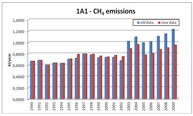
Fig. 3‑15 Development of CH₄ emissions in 1A1 category before and after recalculation

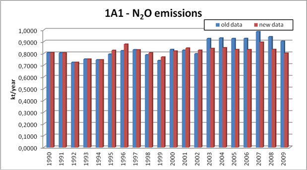
Fig. 3‑16 Development of N₂O emissions in 1A1 category before and after recalculation

There are a number of reasons for the change in the data after 2003. One is the new calorific values of liquid fuels that we obtained in 2011 for the whole time series. The change was obvious for some fuels. Another reason for the decrease in emissions after 2003 consisted in a methodological mistake in the previous inventories; autoproducers were reported in this category. This year we discovered this discrepancy and, together with the recalculation, these consumptions were reallocated to category 1A2. An increase in emissions is then apparent in 1A2 category. A detailed description can be found below under the description of recalculation of category 1A2. A third possible reason for changes in emissions could consist in specification of data directly by CzSO.

Graphs and tables for emission changes in category 1A2 are given below. As mentioned above, similar to the decrease in emissions in category1A1 after 2003, the emissions increase is apparent here. In the initial data files, consumptions for autoproducers are shown as summary values. These values were proportionally divided into individual subcategories 1A2a Iron and Steel, 1A2b Non – Ferrous metals, 1A2c Chemicals, 1A2d Pulp, Paper and Print, 1A2e Food, Beverages and Tobacco and 1A2f Other according to other available indicators, such as development and trends in the relevant branches of industry.

In the previous submissions, all the data in category 1A2 were reported under category 1A2f. Only in 2003 – 2009 were the data reported in each subcategory. In an attempt to extend the data series, the data from the CzSO Questionnaires were used from 1995. However, an effort was made to extend the data series in this category back towards 1990 (in order to have consistent reporting of consumption in all these subcategories as in the other categories – 1A1 and 1A4). Expert estimates were made in 1990 – 1994 according of developments in the relevant branch of industry.

Table 3.24a gives the changes in CO₂ emission before and after the recalculation. No change is apparent before 1994. Table 3.24b shows the changes in emissions after 2003 caused by reallocation of autoproducers as mentioned above.

Tab. 3‑24a Comparison of CO₂ emissions in 1A2 before and after recalculation

1A2 CO₂[Gg]	1990	1991	1992	1993	1994	1995	1996	1997	1998	1999
*Recalculated*
SUM	46 616	49 140	41 106	41 997	32 609	29 405	29 842	29 424	26 377	24 298
Liquid Fuels	9 110	8 218	9 775	7 316	6 072	6 515	6 398	5 914	5 662	5 770
Solid Fuels	31 522	34 338	25 246	27 628	21 348	16 422	16 449	15 844	13 521	11 424
Gaseous Fuels	5 984	6 583	6 084	7 053	5 190	6 468	6 995	7 666	7 193	7 105
Biomass	1 497	1 552	1 555	1 662	1 584	1 738	1 630	1 842	1 786	1 826
Other Fuels

*Before recalculation*
SUM	46 616	49 140	41 106	41 997	32 609	32 766	36 626	29 069	28 588	29 956
Liquid Fuels	9 110	8 218	9 775	7 316	6 072	6 885	7 870	3 962	5 424	7 496
Solid Fuels	31 522	34 338	25 246	27 628	21 348	19 159	20 704	17 529	15 692	15 258
Gaseous Fuels	5 984	6 583	6 084	7 053	5 190	6 722	8 051	7 577	7 472	7 202
Biomass	1 497	1 552	1 555	1 662	1 584	1 590	1 666	1 803	1 386	1 638
Other Fuels

*difference [Gg]*
SUM	0	0	0	0	0	-3 361	-6 784	356	-2 211	-5 658
Liquid Fuels	0	0	0	0	0	-370	-1 472	1 952	238	-1 726
Solid Fuels	0	0	0	0	0	-2 737	-4 255	-1 685	-2 171	-3 835
Gaseous Fuels	0	0	0	0	0	-254	-1 057	89	-278	-97
Biomass	0	0	0	0	0	149	-35	39	399	188
Other Fuels

Tab. 3.24b Comparison of CO₂ emissions in 1A2 before and after recalculation

1A2 CO₂ [Gg]	2000	2001	2002	2003	2004	2005	2006	2007	2008	2009
Recalculated
SUM	28 916	26 785	26 020	25 654	26 437	26 830	26 559	24 163	24 711	23 041
Liquid Fuels	5 339	5 543	5 234	4 814	6 138	6 675	6 249	5 780	6 001	5 575
Solid Fuels	16 646	14 378	13 980	13 980	13 360	13 445	13 619	11 705	12 267	11 998
Gaseous Fuels	6 931	6 864	6 806	6 557	6 578	6 361	6 334	6 376	6 030	5 014
Biomass	1 248	1 456	2 024	1 090	1 322	2 227	2 282	2 417	2 366	2 429
Other Fuels				302	361	349	358	303	413	454

Before recalculation
SUM	28 185	29 432	27 912	18 623	18 576	18 975	17 708	16 845	15 994	15 614
Liquid Fuels	6 164	5 313	4 881	3 704	4 664	4 870	4 170	3 974	3 910	3 532
Solid Fuels	15 214	16 524	15 770	8 721	7 748	8 105	7 428	6 677	6 108	7 100
Gaseous Fuels	6 807	7 594	7 262	5 895	5 803	5 652	5 751	5 891	5 563	4 527
Biomass	1 943	1 940	2 546	971	1 180	1 761	1 823	1 858	1 808	1 807
Other Fuels				302	361	349	358	303	413	454

difference [Gg]
SUM	732	-2 646	-1 892	7 032	7 861	7 855	8 851	7 319	8 717	7 427
Liquid Fuels	-825	230	354	1 110	1 474	1 806	2 078	1 806	2 091	2 043
Solid Fuels	1 432	-2 146	-1 790	5 259	5 613	5 340	6 190	5 027	6 159	4 897
Gaseous Fuels	124	-730	-456	662	775	709	583	485	467	487
Biomass	-695	-485	-522	120	143	466	460	559	558	621
Other Fuels				0	0	0	0	0	0	0

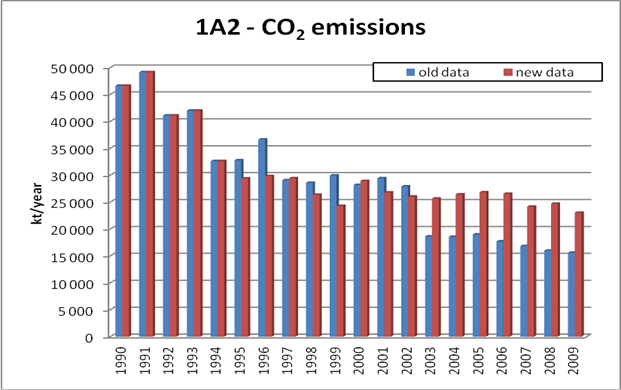
Fig. 3‑17 Development of CO₂ emissions in 1A2 category before and after recalculation

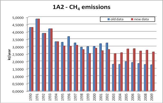
Fig. 3‑18 Development of CH₄ emissions in 1A2 category before and after recalculation

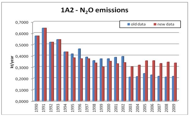
Fig. 3‑19 Development of N₂O emissions in 1A2 category before and after recalculation

This graph (below) shows that total emissions in category 1A didn’t change much after 2003. Thus, the decrease in total emissions in category 1A1 and increase in category 1A2 did not have any overall effect. The small changes are caused by new calorific values, corrections in emission factors and some corrections in the initial data by CzSO.

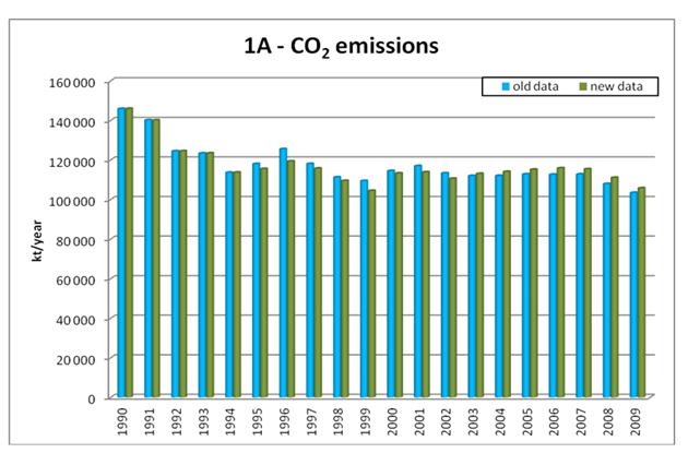
Fig. 3‑20 Development of CO₂ emissions in 1A category before and after recalculation

The next three graphs depict changes in emissions in category 1A4. This category was also recalculated according to the CzSO Questionnaires. The data from the questionnaires were used for calculation of emissions in the 1995 – 2009 period. The data before (1990 – 1994) were left according to the Energy balance of the Czech Republic, which was processed by the CzSO methodology. Good agreement is visible in this category after 2003 (i.e. 2003 – 2009). Where there are some differences, these are because of changes in the emission factors or corrections to the activity data by CzSO. Another discrepancy is caused by the use of different calorific values for liquid fuels during recalculation from kt to TJ. We obtain new calorific values for all the liquid fuels in all the time series from CzSO that were used for calculations during recalculation.

Overall, this can be considered to correspond to very good agreement, as it was expected.

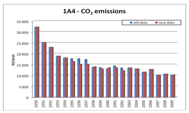
Fig. 3‑21 Development of CO₂ emissions in 1A4 category before and after recalculation

CRF gives comments for all the recalculated categories. The comments are explained below:

AD recalculation 1995 -2009 – for 1A1, 1A4 and 1A3e – Pipeline transport categories; data from CzSO Questionnaires were used for 1995 – 2009. In the previous submission, these data were used only back to 2003 and earlier data were taken from the preliminary energy balance of the Czech Republic. Now these time series were prolonged back to 1995.

AD recalculation 1995 -2009, 1990 – 1994 disaggregation of sum values –for category 1A2 were recalculate whole time series. Data for 1995 – 2009 were taken from the CzSO Questionnaires; summary data were used for 1990 – 1994 (previously all in 1A2f) and these data were proportionally disaggregated into individual categories according to trends in each branch of industry.

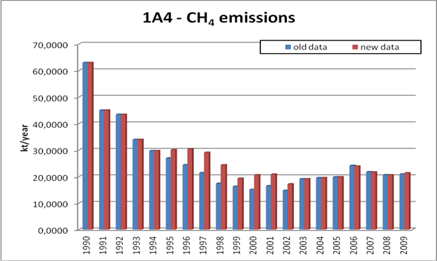
Fig. 3‑22 Development of CH₄ emissions in 1A4 category before and after recalculation

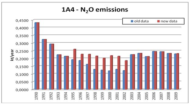
Fig. 3‑23 Development of N₂O emissions in 1A4 category before and after recalculation

AD recalculation 1995 -2009, 1995-1998 expert estimate - used for category 1A5b.

Emission factors

Emission factors were also checked together with the recalculation. The CO₂ emission factors employed were checked with the default emission factors and the consistency in the whole time series was examined. Country-specific EFs were used for Coking Coal, Other Bituminous Coal and Brown Coal – Lignite. Default emission factors were used for the rest of fuels. It was decided to use the default emission factors given by the Revised 1996 IPCC Guidelines for the 1990 – 1994 period and the emission factors given in the 2006 IPCC Guidelines for the 1995 – 2009 period. These emission factors were considered to agree better with the conditions in the Czech Republic and are therefore used consistently in the data series in which the recalculation was performed.

The emission factor for methane was also checked. According to preliminary recommendations, we consistently used the emission factors given in the Revised 1996 IPCC Guidelines. It was not clear whether the emission factor for liquid or for gaseous fuel should be used for LPG - the emission factor for liquid fuels was used in the calculation.

Calorific values

Some differences in values after 2003 could be caused by different calorific values of liquid fuels. In 2011, new calorific values were obtained from CzSO for all the liquid fuels reported in the CzSO Questionnaires. The calculations from kt to TJ were performed using these calorific values, which are almost all different from the previous calorific values.

Reference Approach

The Reference Approach was recalculated in the same way as for the categories in the Sectoral Approach. It was necessary to use the same data source for the Sectoral and Reference Approaches. Thus, the data in the Reference Approach were recalculated according to the CzSO Questionnaires from 1995 to 1999. Some QC activities were also performed during the calculations. It was found that Other fuels are reported in the Reference Approach. It was discovered that these fuels are Other fuels simultaneously reported under 1A2f so they should not be reported again in the Reference Approach. This mistake was corrected in this submission.

One of the repeated recommendations (the last one in CZE_SA-II_2011vers2) was about imports and exports of crude oil for 1990. CRF data for crude oil include net imports while IEA data show imports and exports. Using new calorific values taken from the CzSO Questionnaires (i.e. IEA data), new values were also calculated for import and export for crude oil for the years before 1995. Thus the values for 1990 – 1994 were also changed together with the recalculation after 1995. Consequently, the whole time series was changed for crude oil.

A similar problem was also encountered for export of natural gas in 1990. Exports are reported in the CRF, while they are zero in the IEA data. Export for this year was corrected according to the CzSO Questionnaire. The value in CRF is now zero.

Zero values were discovered for some fuels in the final database. It would be preferable to report these zero exports/imports as a notation key. This methodological mistake will be corrected in next submission. Some inconsistencies in notation keys use will also be corrected in the next submission.

3.7.2 Other Fuels (1A1a) – Recalculations

The entire category is considered to be recalculated for reporting purposes. In fact, this chapter is identical to the previous 6C MSW incineration chapter. In this respect no recalculations were added.

3.7.3 1A3 Mobile Combustion - Source-specific recalculations

In 2010, the data for greenhouse gas emissions in the entire transport sector were recalculated for the 1990 – 2009 time period. The main reason for this recalculation consisted in refinement and harmonization of net calorific values for the whole time period with the KONEKO company and, in some cases, with the IEA – CzSO Questionnaire (CzSO, 2011). The new activity data consequently affected calculation of both transport energy values [TJ] and greenhouse gas emissions.

Several discrepancies relating to the consumption of kerosene in aviation appeared when compared with the IEA database (found by ERT). It was necessary to employ expert engineering assessment, because of the substantial differences in the consumption values in some years. The consumption of kerosene under the administration of KONEKO (other sources) was separated every year from the total consumption of kerosene. The consumption of kerosene under the administration of CDV (international bunkers and civil aviation) was divided into domestic and international aviation on the basis of passengers transport and transport of goods in the whole time period (MTC, 2000; MTC, 2006; MTC, 2011).

The recalculation also encompassed control of values not included in the trends in the monitored GHG. On the basis of the determined results, corrections were performed for 1995 – 2009 (see the elaboration below). The refinement was performed for every category of fuel by supplementing decimal points.

Specification of the adjusted values:

1A3b gasoline correction of energy values and CO₂, CH₄ and N₂O emission values in 1995 – 1999, 2002 – 2006 and 2008

1A3b diesel oil correction of energy values and CO₂, CH₄ and N₂O emission values in 1998 – 2005 and 2008 – 2009

1A3b LPG correction of energy values and CO₂, CH₄ and N₂O emission values in 1995 – 1999

1A3b CNG correction of energy values and CO₂, CH₄ and N₂O emission values in 1995 – 1997 and 2006

1A3c diesel oil correction of energy values and CO₂, CH₄ and N₂O emission values in 1998 – 1999 and 2005

1A3d diesel oil correction of energy values and CO₂, CH₄ and N₂O emission values in 1998 – 1999

3.8 Source-specific planned improvements

3.8.1 Stationary Combustion

The planned improvement consists primarily in a further increase in cooperation with CzSO. As mentioned in the introduction, a new addendum was created for the agreement between the Ministry of the Environment and CzSO. In the framework of this addendum, the parties agreed to hold regular meetings at least 3x annually to deal with coordination of work on the national energy balance, so that this is in accordance with the requirements on processing of activity data for greenhouse gas emission inventories. Simultaneously, the parties agreed to continue in the practice established in 2010 and to hold an annual workshop to discuss in detail current problems and methodical procedures for preparing fuel and emission balances. This effort still remains.

Attention is constantly devoted to obtaining data from the ETS national database for use in performing QA/QC procedures. At the present time, the creation of this database is included in the plan of the Ministry of the Environment. As a certain part of the reports on the individual enterprises are currently available only in printed form, the data cannot be converted as distortion could occur.

It is assumed, that following systematic comparison of activity data obtained in various ways, it will be possible to refine the national GHG inventories in the ENERGY sector using “bottom-up” data, or at least to use this data for the QA/QC procedures.

Another improvement is planned for QA procedures. QA should be performed by an independent expert who does not participate in processing the National Inventory of Greenhouse Gases. It is intended to establish a “working group”, which will consist of independent experts from different branches of industry and energy production. Members of the group should be officially named by a letter of appointment from CHMI as the coordination workplace.

Special attention was paid in 2011 to trends in the country-specific emission factor for Natural Gas. Unfortunately sufficient data were not obtained. Efforts to obtain country-specific emission factors will continue in 2012.

3.8.2 1A3 Mobile Combustion

The planned improvements are related mainly to performance of projects to measure country-specific emission factors in key categories of road transportation. The greatest emphasis will be placed on acquisition of sufficient data for CO₂ and N₂O emission calculation and refinement of methodologies for each category of transport.

3.9 Fugitive emissions from solid fuels and oil and Natural Gas (1B)

Mining, treatment and all handling of fossil fuels are sources of fugitive emissions. In the Czech Republic, CH₄ emissions from underground mining of Hard Coal are significant, while emissions from surface mining of Brown Coal, Oil and Gas production, distribution, storage and distribution are less important.

The current inventory includes CH₄ emissions for the following categories:

1B1 Solid fuels
1B2 Oil and Natural Gas

In 1B Fugitive Emissions from Fuels category, especially 1B1a Coal Mining and Handling was evaluated as a key category (Table 3.25). Category 1B2 also was identified as a key category by the latest assessment, but only in one from the four tests (LA). Moreover, identifiers placed this category just over the borderline between key and non-key categories.

Fig. 3‑24 depicts methane emissions trends from selected categories from the sector 1B Fugitive Emissions from Fuels.

Tab. 3‑25 Overview of significant categories of sources in this sector (2010)

Category	Character of category	Gas	% of total GHG*
1B1a Fugitive Emissions from Coal Mining and Handling	KC (LA, TA, LA, TA)	CH₄	2.4
1B2 Fugitive Emissions from Oil & Gas operations	KC (LA, LA*)	CH₄	0.5

* assessed without considering LULUCF (without * means considering LULUCF)

KC: key category, LA: identified by level assessment, TA: identified by trend assessment

Fig. 3‑24 Methane emissions trends from the sector Fugitive Emissions from Fuels [Gg CH₄]

3.9.1 Solid Fuels (1B1)

The source category 1B1 Solid Fuels consists of three sub – source categories: source category 1B1a

Coal mining and Handling, source category 1B1b Coal transformation and source category 1B1c Other.

The main process that emits more than 80 % of methane emissions from the category 1B1Solid Fuels category is underground mining of Hard Coal in the Ostrava-Karviná area. A lesser source consists in Brown Coal mining by surface methods and post-mining treatment of Hard and Brown Coal. Coal mining (especially Hard Coal mining) is accompanied by an occurrence of methane. Methane, as a product of the coal-formation process is physically bonded to the coal mass or is present as the free gas in pores and cracks in the coal and in the surrounding rocks.

Abandoned mines

In the Czech Republic there are also abandoned mines occurring. All of them have CH₄ recovery systems. There is company, which has established mining areas for mining of fire-damp in Ostrava-Karviná area. In the abandoned mines there are automatic suction devices and firedamp stations. Firedamp arises from abandoned mining pits and surface boreholes into abandoned areas. Mined firedamp is used at the place of mining in autonomous cogeneration units (aggregate for electricity energy production with an ignition combustion engine)( http://www.dpb.cz/).

3.9.1.1 Source category description

1B1a Coal mining and Handling

In underground Hard Coal mining, CH₄ is released from the coal mass and from the surrounding rocks into the mine air and must be removed to the surface to prevent formation of dangerous concentrations in the mine.

1B1a1 Underground Mines

In the Czech Republic, mainly Hard Coal is mined in underground mines (i.e. Hard Coal: Coking Coal and Bituminous Coal). Presently, underground mines are in operation in the Ostrava-Karviná coalmining area. In the past, Hard Coal was also mined in the vicinity of the city of Kladno. These mines were closed in 2003. Brown Coal is mined in only one underground mine in the Northern Bohemia. Emissions from this mine are reported together with surface mining of Brown Coal – Lignite in subcategory 1B1a2 Surface Mines.

1B1a11 Mining Activities

The data of CzSO in the report CZECH_COAL.xls (CzSO, 2011) can be used for control purposes.

Hard-coal mining is the principal source of fugitive emissions of CH₄. The mine ventilation must be regulated according to the amounts of gas released to keep its concentration on safe level. At the end of 1950’s mine gas removal systems were introduced in opening new mines and levels in the Ostrava- Karviná coal-mining area, which permitted separate exhaustion of partial methane released in the mining activity in the mixture containing the mine air. The total amount of methane emitted can be balanced quite accurately from the methane concentrations in the mine air and their total annual volume.

1B1a12 Post-Mining Activities

The activity data are the same as in category 1B1a11 Mining Activities. It is assumed that the entire mined volume undergoes manipulation during which residual methane is released.

1B1a2 Surface Mines

1B1a21 Mining Activities

Brown Coal and Lignite are mined in surface mines in the Czech Republic. Brown Coal is mined primarily in the Northern Bohemia area, while Lignite mines are located in Southern Moravia.

1B1a22 Post-Mining Activities

The activity data are the same as in category 1B1a21 Mining Activities. It is assumed that the entire mined volume undergoes treatment during which residual methane is released.

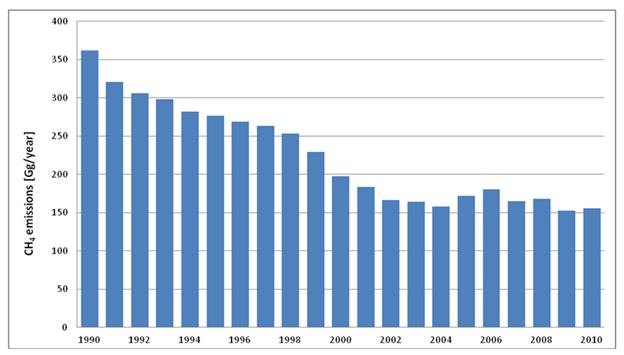
Fig. 3‑25 Methane emissions trends from the sector Fugitive Emissions from Solid fuels [Gg CH₄]

1B1b Coal transformation

The subcategory includes

a) production of Coke from Coking Coal

Fugitive methane emissions from coal treatment prior to the actual coking process are listed under 1B1a12 Post-Mining Activities. Emissions from the actual production of Coke are given under 2. Industry.

b) production of briquettes from Brown Coal

Fugitive methane emissions from coal treatment prior to the actual briquetting process are listed under 1B1a22 Post-Mining Activities. CO₂ emissions from the actual production of briquettes are included in subcategory 1A2f.

For these reasons, none of the activity data or methane emissions are included in this subcategory

(notation key IE). Fugitive CO₂ emissions are not estimated or are negligible and no known method is available for their determination (notation key NE). Fugitive N₂O emissions are not estimated because, according to the current state of knowledge, these emissions cannot occur (notation key NA).

1B1c Other

No other subcategory of fugitive methane emissions is known in the Czech Republic.

3.9.1.2 Methodological issues

1B1a1 Underground Mines

1B1a11 Mining Activities

National emission factors were determined for calculation of fugitive methane emissions in underground mines in the second half of the 1990’s: the ratio between mining and the volume of methane emissions is given in Table 3.26, see (Takla and Nováček, 1997).

Tab. 3‑26 Coal mining and CH₄ emissions in the Ostrava - Karvina coal-mining area

	Coal mining	CH₄ emissions	Emission factors
	*[mil. t / year]*	*[mil. m³ / year]*	*[m³ / t]*
1960	20.90	348.9	16.7
1970	23.80	589.5	24.7
1975	24.11	523.8	21.7
1980	24.69	505.3	20.5
1985	22.95	479.9	20.9
1990	20.6	381.1	19.0
1995	15.60	270.7	17.4
1996	15.10	276.0	18.3
Total	167.31	3 375.3	20.2
1990 till 1996	50.76	927.8	18.3

Only the values for 1990, 1995 and 1996 were used from this table to determine the emission factors.

The average value of the emission factor of 18.3 m³/t was recalculated to 12.261 kg/t using a density of methane of 0.67 m³/kg. This emission factor is used for coal mined in the Ostrava-Karviná coalmining area for years 1990 - 1999. The emission factor set by estimation at 50 % of this value was used for the remaining Hard Coal from deep mines in other areas. This is valid for coal with minimum coal gas capacity (coal from the Kladno area to 2002 and coal from the Žacléř area from 1998).

The emission factors given in table 3.30 in the recalculation chapter are used for 2000 – 2008. After 2008, the emission factor calculated as the average value from the values for 2000-2008, i.e. 8.12 t/kt, is used. According to the ERT recommendation, a survey was performed to update these emission factors, which consequently caused other recalculation which are described in detail in the relevant chapter

1B1a12 Post-Mining Activities

Methane emissions in the subcategory of Post-Mining Activities are calculated using a uniform emission factor based on the default value of 1.64 kg CH₄/t coal; the activity data are employed at the same level as in subcategory 1B1a11 Mining Activities.

Tab. 3‑27 contains a summary of fugitive methane emissions during the actual underground mining of Hard Coal and during post-mining operations.

Tab. 3‑27 Used emissions factors and calculation of CH₄ emissions from underground coal mining in 2010

	Amount of Coal	Emission	Methane
	Produced	Factor	Emissions
	[million t]	[kg CH₄/t]	[Gg CH₄]
OKR^) (tier III)*	11.001	8.8	96.3
Other - tier I	0.000	6.7	0.0
Mining (tier III)	11.001	8.8	96.3
OKR^) (tier I)*	11.001	1.6	18.1
Other - tier I	0.000	0.6	0.0
Post-Mining (tier I)	11.001	1.6	18.1
Total sub-sector 1B1a1	11.001	10.4	114.3

* Ostrava-Karviná coal-mining area

1B1a2 Surface Mines

1B1a21 Mining Activities

Data from the source part of the questionnaire completed in the CzSO Questionnaire (CzSO, 2011), was employed to determine activity data on extraction of Brown Coal and Lignite. The mining yearbooks and other data sources continue to be used only for control purposes.

During surface mining, escaping methane is not related to specific flow of air and thus it is far more difficult to monitor the amount of methane escaping into the air. Consequently, default IPCC emission factors are employed to calculate methane emissions from surface mining and from post-mining treatment (IPCC, 1997).

Table 3.20 illustrates the calculation of fugitive emissions of methane from surface coal mining activities.

Tab. 3‑28 Emission factors employed and calculation of CH₄ emissions from surface coal mining in 2010

	Amount of Coal	Emission	Methane
	Produced	Factor	Emissions
	*[million t]*	*[kg CH₄/t]*	*[Gg CH₄]*
Mining (tier I)	43.774	0.77	33.7
Post-Mining (tier I)	43.774	0.07	2.93
Total sub-sector 1B2a1	43.774	0.84	36.63

3.9.1.3 Uncertainty and time-series consistency

The inventory methods used in this inventory were consistently employed across the whole reporting period from the base year of 1990 to 2010.

The uncertainties in the activity rate result primarily from inaccuracies in weighing of extracted coal.

Uncertainties in determining the activity data are estimated at 5 %.

Uncertainties in calculating methane emissions further follow from the emission factors employed.

The emission factors for determining emissions from deep mining of hard coal are based on measurement of the methane concentrations in the air ventilated from underground mines in the second half of the 1990’s. The precision of methane emissions varies at a level of 5 %. The uncertainty in the default emission factors is considered to be at a level of 80 %. Overall, the uncertainty in the emission factors in category 1B1 Solid fuels is estimated to equal 40 %.

Consistency of the time series is apparent from the graphs in Fig. 3‑24. Minor fluctuations are caused by climatic variations in the individual years. The trends towards a substantial decrease in emissions in the 1990’s decreased during the first decade of the 21^st century.

3.9.1.4 Source specific QA/QC and verification

General quality control and source-specific quality control (Tier 1 and Tier 2), in conformance with the requirements of the QSE handbook and its associated applicable documents, have been performed to the full extent.

QC activities at the level of Tier 1 were performed according to the QA/QC plan by the sector compiler. Routine control was performed in the framework of the following activities:

activity data employed,
emission factors employed,
calculation procedures employed,
transfer of numerical data from the working set to the CRF Reporter.

During control of the activity data, the CzSO data were compared with the data from the Mining Yearbook. Good agreement was found.

In control of the emission factors employed, the emission factors used in the Czech Republic methodology were compared with the emission factors of Slovakia, Poland and Germany in the context with the default emission factors. It was found that the emission factors employed for calculation of emissions in the Czech Republic methodology correspond, in their range, to the emission factors employed in the other countries. Comparison of the emission factors used in the

Czech Republic with the emission factors of the surrounding countries corresponds to the level of Tier 2.

Control that the transfer of numerical data from the working set to the CRF Reporter does not reveal any differences. The final working set in EXCEL format is locked to prevent intentional rewriting of values and archived at the coordination workplace. The protocols on the performed QA/QC procedures are stored too.

3.9.1.5 Source-specific recalculations

1B1a – Coal Mining and Handling

Two recalculations were performed on the basis of ERT recommendations.

A. Recalculation of CH₄ emissions from underground mining of hard coal

Recalculation was performed on the basis of a recommendation in FCCC/ARR/2008/CZE of March 25 2009 in paragraph 37. This recommendation suggests that the CH₄ emission factor for underground coal mining be updated.

In connection with this requirement, the management of OKD, a.s. (Ostrava-Karviná mines, joint share company) was contacted. The company monitors in very detail the problematic about methane production. In response to a request from the reporting team, the company provided a document in which the total amount of gas released by OKD mines was determined, together with the amount of methane withdrawn by degassing, the amounts of methane used for industrial purposes, venting of methane from degassing and the total amount of methane released into the atmosphere.

Tab. 3‑29 Methane production from gas absorption of mines and its use

	*mil.m³ CH₄ year^-1**
year	total amount	pumped out by	industrial	venting from gas absorption	released into the
	of gas	gas absorption	use	into the atmosphere	atmosphere - total
2000	236.7	84.1	77.9	6.2	158.8
2001	210.7	73.9	71.1	4.0	140.8
2002	210.0	81.0	70.3	1.3	130.3
2003	200.6	74.8	72.8	2.0	127.8
2004	194.6	77.1	73.4	3.2	120.7
2005	207.7	73.9	70.3	3.6	137.4
2006	221.1	76.9	75.9	0.8	145.0
2007	194.7	71.5	71.0	0.5	123.7
2008	199.5	68.8	68.5	0.3	131.0

This information was used to calculate the emission factors and to determine the average emission factor, which is used for the period after 2000-2008.

Tab. 3‑30 Calculation of emission factors from OKD mines for period 2000 onwards

year	OKD mining	CH₄ emissions	EF
	[kt/year]	[t/year]	[t/kt]
2000	11 514	106 396	9.24
2001	11 844	94 336	7.96
2002	12 049	87 301	7.25
2003	11 301	85 626	7.58
2004	10 901	80 869	7.42
2005	10 822	92 058	8.51
2006	11 656	97 150	8.33
2007	10 153	82 879	8.16
2008	10 030	87 770	8.75
2000 - 2008	100 270	814 385	8.12

For years 2000 – 2008 were used emission factors given in table for calculation of emission factors from OKD mines. For years onwards 2008 is used average emission factors from the period 2000-2008; 8.12 t/kt of mined hard coal, for period before 1999 the value is same as in previous submission 12.3 t/kt of mined coal (Takla and Nováček, 1997).

This emission factor can be considered as emissions factor on the level Tier III – it is country-specific emission factor, which is applicable for Ostrava-Karviná area.

For other mines in the Czech Republic where hard coal was also mined, the value of 6.7 t/kt was used – the same as in previous submissions. However it is necessary to remind that underground mining in the mines of other areas than OKD is really minor and at the end of the first decade of 21^st century was completely stopped.

In comparison with the previous submission, the recalculation leads to lower CH₄ emissions after 2000. Comparison of the primary values from the whole subsector 1B1 Solid Fuels (Coal Mining and Handling) can be seen in the figure.

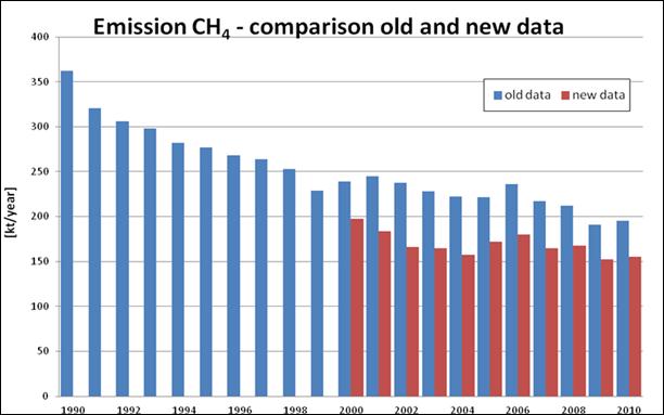
Fig. 3‑26 Source: Hok Petr: “Účelový materiál pro řešení inventarizace skleníkových plynů o emisích metanu z dolů OKD v letech 2000 až 2008, OKD, a.s., Ostrava 28. 8. 2009”[13]

B. New data about CO₂ emissions from underground mining of hard coal

A recommendation to estimate CO₂ emissions for underground and surface coal mining followed from FCCC/ARR/2010/CZE of February 16 2011 (paragraph 41) and from the response of ERT to the in-country review in August/September 2011 in Prague .

Calculation of CO₂emissions for underground mining was considered to be a priority. It was necessary to calculate new data for CO₂ emissions from underground hard coal mining. This calculation was based on the fact that the mine drainage gas also contained CO₂. Both gases (CH₄ and CO₂) represent a danger for human health in mines and are therefore monitored and their amounts in mine drainage gas are evaluated. An extra study was performed to determine the CO₂ emission factor for underground hard coal mining. Monthly data on the concentrations and amounts of CO₂ were processed for all the exhaust air shafts in the OKD area for 2009, 2010 and for part of 2011. These data yielded an average value of the emission factor, which is related to the volume of mining. The emission factor is equal to 22.75 t/kt of mined coal and this emission factor is country specific – Tier III level. This value is valid for the OKD area. The author of the study recommended that the determined emission factor for 1990 – 2009 be used. He determined an emission factor 22.68 t/kt of mined coal for 2010 and it was recommended that this value also be used for the subsequent years.

These emission factors were used to extend the data for CO₂ emissions for underground hard coal mining; the values are given in the table.

Tab. 3‑31 Emission factors and emissions from deep mining of hard coal

	production	emission	emission of
year	OKD	factor	CO₂
	[kt/year]	[t/kt]	[kt CO₂/year]
1990	20 059	22.75	456.3
1991	17 371	22.75	395.1
1992	17 271	22.75	392.9
1993	16 419	22.75	373.5
1994	15 942	22.75	362.6
1995	15 661	22.75	356.2
1996	15 109	22.75	343.7
1997	14 851	22.75	337.8
1998	14 620	22.75	332.6
1999	13 468	22.75	306.4
2000	13 855	22.75	315.2
2001	14 246	22.75	324.1
2002	14 200	22.75	323.0
2003	13 614	22.75	309.7
2004	13 272	22.75	301.9
2005	13 227	22.75	300.9
2006	14 280	22.75	324.8
2007	12 886	22.75	293.1
2008	12 622	22.75	287.1
2009	11 001	22.75	250.2
2010	11 435	22.68	259.3

Source: Prokop Pavel: Zpracování emisních faktorů a emisí CO₂ při hlubinné těžbě černého uhlí v OKR, Technická univerzita Ostrava, Ostrava, říjen 2011

Consultations with experts on surface mining showed that similar data for determination of CO₂ emissions are not available. However, experience from an area where surface mining was recently active suggests that the amount of CO₂ released by lignite - brown coal mining is absolutely minor.

Comments are given in CRF for the recalculated categories. Explanation of comments is given below:

Note raised by ERT during ICR 2011 – used for 1B1A11 Mining Activities, CH₄ Emissions – Recovery. During the in-country review in September 2011, a question was raised about recovery from abandoned mines. We pointed out that abandoned mines exist in the country and that all of them have CH₄ recovery systems. The recommendation was to elaborate in next annual submission how the recovered CH₄ emissions from each abandoned mine are treated. Consequently, it is not possible to leave notation key NO in the CRF Reporter.

Update - used for 1B1A11 Mining Activities, CH₄ Emissions 2000 – 2009. This change follows from a recommendation raised in document FCCC/ARR/2008/CZE (March 25 2009), paragraph 37, where it is recommended to update the CH₄ emission factor for underground mines – mining activities.

Available new AD - used for 1B1A11 Mining Activities, CO₂ Emissions 1990 – 2009. This recommendation was raised in FCCC/ARR/2010/CZE (February 16 2011), paragraph 41 and by ERT during the in-country review in September 2011. It was recommended to estimate CO₂ emissions from underground mining and surface mining.

3.9.1.6 Source-specific planned improvements

No improvements are planned at the present.

3.9.2 Oil and Natural Gas (1B2)

Source category 1B2 Oil and Natural Gas consists of four source subcategories: source category 1B2a

Oil, source category 1B2b Natural Gas, 1B2c Venting and flaring and source subcategory 1B2d Other.

Approximately 10 % of emissions are formed in the Czech Republic from gas industry in extraction, storage, transport and distribution of Natural Gas and in its final use. Crude Oil extraction and refining processes are less important.

Determination of methane emissions from the processes of refining of Crude Oil is based on the recommended (default) emission factors according to the IPCC methodology.

Methane emissions from the gas industry were determined using national emission factors based on the specific emission factors for the individual parts of the gas industry system (Alfeld, 1998).

The graph in Fig. 3‑27 gives an overview of the trend in emissions in this category in the time series since 1990.

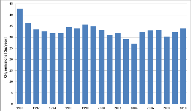
Fig. 3‑27 Methane emissions trends from the sector Fugitive Emissions from Oil and Natural Gas [Gg CH₄]

3.9.2.1 Source category description

1B2a Oil

CH₄ emissions from Crude Oil transport and refining and from Crude Oil mining, which is performed in the Czech Republic in combination with mining of Natural Gas, are reported in this category. CO₂ emissions from the refinery resulting from combustion processes (including flaring) are included in

1A1b Crude Oil Refining.

1B2a1 Exploration

Exploration is not systematically performed in the Czech Republic.

1B2a2 Production

Crude Oil is mined in the Czech Republic in Southern Moravia. The following table gives the amount of mined Crude Oil in the territory of the Czech Republic.

Tab. 3‑32 Crude Oil mining in the CR in 2000 – 2010

Year	2000	2001	2002	2003	2004	2005	2006	2007	2008	2009	2010
[kt/year]	175	183	265	317	306	313	265	246	242	222	176

1B2a3 Transport

Transport of Crude Oil in the territory of the Czech Republic is performed only in closed systems (pipeline transport). So far, emissions from this subsector have not been evaluated. In the context of internal control procedures, this fact was identified as an inadequacy and thus default emission factors were sought for CH₄ and CO₂ emissions and were used to calculate fugitive emissions in this subsector.

1B2a4 Refining / Storage

Crude Oil is processed in the territory of the Czech Republic in two main refinery facilities. Tab. 3‑33 gives the total volume of Crude Oil processed in the Czech Republic.

Tab. 3‑33 Total Crude Oil input to rafineries in CR in 2000 – 2009 [kt/year]

Year	2000	2001	2002	2003	2004	2005	2006	2007	2008	2009	2010
Refinery Intake	5 871	6 072	6 238	6 573	6 704	7 746	7 866	7 394	8 249	7 376	7 901

1B2a5 Distribution of oil products

The final products after processing Crude Oil no longer contain dissolved methane or carbon dioxide and thus fugitive emissions are not considered in this subcategory. For completeness, activity data corresponding to the volume of processed Crude Oil in the individual years were recorded in CRF.

1B2a6 Other

No other operations are considered.

Tab. 3‑34 summarizes the activity data and emission factors used, including calculation of total methane emissions in this subcategory.

		A	B	C	D
Category	Tier	Activity	Emission Factors	CH₄ Emissions	Emissions CH₄
				(kg CH₄)	(Gg CH₄)
				C = (A x B)	D = (C/10⁶)
Production - OIL		PJ oil produced	kg CH₄/PJ
*domestic production*	3	7.46	5 287	39 441	0.039
Transport		PJ oil refined	kg CH₄/PJ
*transport of Crude Oil*		335	146	48 910	0.049
Refining		PJ oil refined	kg CH₄/PJ
*processing of Crude Oil*	1 - 2	335	1 150	385 250	0.385
				CH₄ from Oil	0.474

1B2b Natural Gas

1B2b1 Exploration

Emissions formed at exploratory boreholes are reported in this subcategory. This activity is not performed in the Czech Republic, or is completely random.

1B2b2 Production

Natural Gas is extracted in the Czech Republic in the area of Southern Moravia, accompanying extraction of Crude Oil, and in Northern Moravia, where it is derived from degassing of hard coal deposits. The following Tab. 3‑24 gives the amount of extracted Natural Gas in the territory of the Czech Republic.

Tab. 3‑35 Extraction of Natural Gas in the CR in 2000 - 2010

Year	2000	2001	2002	2003	2004	2005	2006	2007	2008	2009	2010
[mill. m3/year]	219	160	153	168	215	201	194	201	199	178	203

This subcategory contains estimations of emissions formed during the actual technical operations during mining, with the exception of venting and flaring.

1B2b3 Transmission

A transit gas pipeline runs through the territory of the Czech Republic, transporting Natural Gas from Russia to the countries of Western Europe, with a length of 2,455 km. In addition to this central gas pipeline, a system of high-pressure gas pipelines is in operation in the territory of the Czech Republic, providing supplies of Natural Gas from the transit gas pipeline and underground gas storage tanks to centres of consumption. In 2010, the high-pressure gas pipelines had an overall length of 16 645 km.

This length is gradually increasing. This subcategory also includes all the technical equipment on high-pressure gas pipelines. On the transit gas pipeline, this consists primarily of compressor stations and transfer stations, while measuring and regulation stations are located on domestic long-distance gas pipelines.

Emissions formed during controlled technical discharge of Natural Gas at compressor stations, during inspections and repairs to pipelines and emissions from pipeline accidents are estimated. These emissions are recorded by the gas companies. In addition, escapes of Natural Gas from leaks in the entire pipeline system, including technical equipment, are also evaluated.

1B2b4 Distribution

Emissions from distribution gas pipelines, with an overall length in 2010 of 59 190 km, and during consumption at the end consumer are reported in this category. The distribution networks are being continuously lengthened and the number of customers is increasing.

1B2b5 Other Leakage – 1B2b51 at industrial plants and power stations

Emissions from storage (injection and mining) of Natural Gas in the territory of the Czech Republic are reported in this subcategory. The total turnover (injection and mining) of Natural Gas in underground storage areas corresponded to 2 781 mil. m³ in 2010.

1B2b5 Other Leakage – 1B2b52 in residential and commercial sectors

No emissions were identified in subcategory 1B2b52 Other leakage in the residential and commercial sectors in the Czech Republic and thus the notation NO is employed.

Activity data, emission factors and the resultant emission data are given in Table 3.26 for the entire 1B2b Natural Gas sector.

Tab. 3‑36 Calculation of CH₄ emissions from Gas in 2010 in structure IPCC

		A	B	C	D
Category	Tier	Activity	Emission Factors	CH₄ Emissions	Emissions CH₄
				(kg CH₄)	(Gg CH₄)
				C = (A x B)	D = (C/10⁶)
Production/Processing		PJ gas produced	kg CH₄/PJ
*(domestic production NG)*	3	6.91	39 354	272 020	0.272
Transmission and Storage		PJ gas transported	kg CH₄/PJ
*(transit transport and high press pipeline)*	2	1 356.60	10 088.16	13 685 599	13.69
Distribution		PJ gas distributed	kg CH₄/PJ
*(low pressure pipeline)*		163.76	109 937.15	18 002 757	18.00
Other Leakage		PJ gas stored	kg CH₄/PJ
*(underground storage)*	3	94.68	14 758	1 397 252	1.4
		TOTAL CH₄ from Gas			33.36

1B2c Venting and Flaring

In this category the default EFs from the IPCC Good Practice Guidance (table 2.16, pages 2.86-2.87) were used. The EF value of 2.7 E-04 Gg per 103 m³ was used for conventional oil production, which was taken from the “Oil Production, Conventional Oil, Fugitives” part of table. Owing to the fact that activity data are required in kg/PJ, the value was converted to 7 327.9 kg/PJ by using the typical value of density for crude oil of 880 kg/t and NCV = 41.87 MJ/kg (this value was calculated as the weighted average for the 1990 – 2008 period from the CzSO questionnaires for IEA).

In addition, the estimations of CO₂, CH₄ and N₂O emissions from venting and flaring in the course of oil production were obtained by using the default EFs provided by the IPCC Good Practice Guidance (see table 2.16, page 2.86). In this case the following EFs were taken (from the part of the table for “Oil Production, Conventional Oil, Venting and Oil Production, Conventional Oil, Flaring”):

1. B. 2. c. Venting

CH₄: 6.2E-05 to 270E-05 Gg per 103 m³ conventional oil production

CO₂: 1.2E-05 Gg per 103 m³ conventional oil production

1. B. 2. c. Flaring

CH₄: 0.5E-05 to 27E-05 Gg per 103 m³ conventional oil production

CO₂: 6.7E-02 Gg per 103 m³ conventional oil production

N₂O: 6.4E-07 Gg per 103 m³ conventional oil production

As in the previous case (1.B.2.a.ii), the EFs were converted to kg/PJ by using the same values for the oil density and NCV.

For CH₄, only the minimum and maximum values of the EF range are given. Taking into account that the range is rather wide, we assumed lognormal distribution; see 2006 IPCC Guidelines, Vol. 1: General Guidance and Reporting, Chapter 3.2.2.4 Good practice guidance for selecting probability density functions, p. 3.23. Therefore, the average of the logarithms was used for evaluation of the EFs for venting and flaring:

1. B. 2. c. Venting

CH₄: 11 104 kg/PJ

CO₂: 325.7 kg/PJ

1. B. 2. c. Flaring

CH₄: 997.2 kg/PJ

CO₂: 1 818 399 kg/PJ

N₂O: 17.4 kg/PJ

Table 3.38 gives the CH₄ and CO₂ emissions from Venting for domestic extraction of petroleum; N₂O emissions are not included in this subcategory since no emission factor is available for their calculation.

Table 3.38 further contains CH₄, CO₂ and N₂O emissions from Flaring in domestic extraction of petroleum.

Tab. 3‑37 Emissions of CH₄, CO₂ and N₂O from Venting and Flaring in 1990 – 2010

	Venting - emissions [t/year]		Flaring - emissions [t/year]
	CH₄	CO₂	CH₄	CO₂	N₂O
1990	23.4	0.688	2.1	3 839	0.037
1991	31.5	0.924	2.8	5 162	0.049
1992	37.7	1.107	3.4	6 180	0.059
1993	51.0	1.495	4.6	8 346	0.080
1994	59.4	1.744	5.3	9 735	0.093
1995	67.5	1.974	6.1	11 022	0.105
1996	70.3	2.055	6.3	11 476	0.110
1997	75.4	2.204	6.8	12 306	0.118
1998	82.7	2.419	7.4	13 505	0.129
1999	85.2	2.490	7.6	13 904	0.133
2000	81.6	2.385	7.3	13 317	0.127
2001	85.2	2.492	7.7	13 911	0.133
2002	123.6	3.614	11.1	20 176	0.193
2003	147.6	4.316	13.3	24 099	0.230
2004	142.2	4.159	12.8	23 220	0.222
2005	145.5	4.254	13.1	23 751	0.227
2006	123.5	3.612	11.1	20 168	0.193
2007	114.9	3.361	10.3	18 764	0.179
2008	112.9	3.300	10.1	18 425	0.176
2009	103.5	3.037	9.3	16 902	0.161
2010	82.9	2.430	7.4	13 570	0.130

3.9.2.2 Methodological issues

1B2a Oil

During the 1990’s, Czech refineries have undergone a quite extensive process of innovation and reconstruction, to decrease technical losses of raw materials and final products. Comprehensive verification has been carried out of the seals of the individual fittings, pumps and all the technical equipment. This entire process, which was carried out mainly for economic reasons, also led to a decrease in overall emissions, especially of NMVOCs. Consequently, the emission factors taken from the IPCC methodology (IPCC, 1997) can be considered to correspond to the current technical condition of refineries in this country. In this connection, it should be pointed out that fugitive emissions from refinery technology couldn’t be determined by direct measurements, as they are not connected with specific air outlets or chimneys. Thus, they can be determined only on the basis of professional estimates from balance losses or using emission factors. The resultant emissions of the individual substances were compared with the data in the national emission database and are of the same order of magnitude.

In general, it can be stated that fugitive greenhouse gas emissions occur in this subcategory only in operations in which Crude Oil saturated in carbon dioxide and methane is in contact with the atmosphere. All operations involving Crude Oil in the Czech Republic are hermetically sealed. Thus, fugitive emissions are formed only through leaks in the technical equipment. Following thermal treatment of Crude Oil, the resultant products no longer contain any dissolved gases and no fugitive emissions need be considered in subsequent operations.

1B2a1 Exploration

Activity data: number of mined boreholes – notation key NO, default emission factors have not been published for CO₂ and CH₄ – notation key NO; this notation key was corrected in this submission on the basis of an ERT (in-country review 2011) recommendation. N₂O emissions: notation key NA: N₂O emissions are practically not formed in exploratory work.

1B2a2 Production

Activity data for determining CH₄emissions are taken from the CzSO – IEA questionnaires and controlled using data from the Mining Yearbook. CH₄ emissions are determined as the product of annual Crude Oil mining and the emission factor. The emission factor has a value of 5,287 kg/PJ and was determined on the basis of published data in (Zanat et al.,1997). The emission factor was determined as the sum of the individual emission factors from pumping of raw Crude Oil and from storage of raw Crude Oil. These data were obtained by direct measurement. The resultant emission factor was increased by an estimate of fugitive emissions at mining boreholes (probes).

1B2a3 Transport

In this case, the activity data correspond to the total amount of petroleum transported through the territory of the Czech Republic by the pipeline system in the individual years. This amount corresponds to the Total Crude Oil input to refineries. The default emission factors from IPCC Good

Practice Guidance Table 2.16, page 2.87 are employed to calculate the CH₄and CO₂ emissions.

EF CH₄ – 0.00015 kt/PJ, EF CO₂ – 0.00001 kt/PJ. These emission factors were used to calculate fugitive emissions for the years since 1990.

1B2a4 Refining / Storage

Methane emissions from refining are calculated using IPCC Tier 1 methodology (Table 4.2.4 in 2006 IPCC Guidelines for National Greenhouse Gas Inventories). Emissions are calculated by multiplying the amount of Crude Oil input to refinery by the emission factor. The emission factor value used was 1,150 kg/PJ.

The IPCC method does not give any EF for CO₂ or N₂O. Consequently, the notation key NE is used in CRF.

1B2a5 Distribution of oil products

The available IPCC methodology does not provide any EF for CO₂, CH₄ or N₂O – notation key – NE. The products which originate during oil processing cannot contain CO₂ or CH₄. There isn’t known process by which could arise fugitive CO₂ or CH₄ emissions during the distribution of oil products.

1B2a6 Other

Activity data: notation key: NO; CH₄ and CO₂ emissions – notation key NO.

1B2b Natural Gas

Leakages in the distribution network and household distribution pipes can be considered to constitute the most serious source of emissions. In the 1990's, the distribution network was newly constructed almost entirely from welded plastics and the old pipeline was reconstructed to a major degree in the same manner. Household distribution pipes are subject to strict standards and any poor seals can be identified by the characteristic smell. In addition to safety aspects, all leakages also have an economic impact both for the distribution company and for the end user, so this aspect is carefully monitored and, as soon as possible, immediately remedied. As a whole, the gas distribution in the CR is at a high technical level and it can be stated that all leakages are carefully sought out and eliminated.

As a method was developed in the last few years for determining methane emissions in the gas industry using specific emission factors, this sophisticated method of calculation continues to be used, although, from the standpoint of ref. (Good Practice Guidance, 2000), calculation using default values would probably suffice. Qualified estimation of methane emissions is thus carried out using specific emission factors for the individual parts of the gas industry system (Alfeld, 1998). The total emission value given corresponds to about 0.3 % of the total consumption of Natural Gas in the Czech Republic. The detailed calculation given corresponds to Tier 2.

In general, it can be stated that the determined methane emissions in category 1B2 Gas are basically formed in several ways:

· through poor seals in the flanges and joints, fittings, probes in mining and storage fields and other parts of the pipeline system,

· through pipeline perforation,

· through technical discharge of gas into the air,

· through accidents.

1B2b1 Exploration

Exploration is not performed in the Czech Republic and thus the notation key NO is used in the CRF Report for the emissions and activity data.

· 1B2b2 Production

· 1B2b3 Transmission

· 1B2b4 Distribution

· 1B2b5 Other Leakage – 1B2b51 storage of Natural Gas

Fugitive methane emissions are calculated in these subcategories using an internal calculation model based on the methodology proposed in 1997 in IGU (Alfeld, 1998). Calculations of emissions are supplemented by data from the national Integrated Pollution Register (IPR) and investigations at individual distribution companies on registered units of Natural Gas.

Tab. 3‑38 Model calculation of CH₄ emissions in the Natural Gas sector (2010)

	EF		Activity data		Emissions
	value	units	value	units	mil.m³/year
production	0.20	% vol.	203.0	mil. m³	0.406
high pressure pipelines	600	m³/km.year	16 645	km	9.987
compressors					10.439
storage	0.075	% vol.	2 781	mil. m³	2.085
regulation stations	1 000	m³/station	4 432	pcs	4.432
distribution network	300	m³/km.year	59 190	km	17.757
final comsumption	2	m³/consumer	2 340 339	pcs	4.681
Total					49.79
	Emissions in Gg (0.67 kg/m³)				33.36

Emissions calculated in this model are then transformed to the structure of the sectors and subsectors according to the IPCC methodology.

3.9.2.3 Uncertainty and time-series consistency

The inventory methods used in this inventory were consistently employed across the whole reporting period from the base year of 1990 to 2009.

Uncertainties in determining the activity data are estimated at 5 %. This estimate is based on the precision of measurement of the volumes of Crude Oil, Crude Oil products and Natural Gas.

Uncertainties in calculating methane emissions further follow from the emission factors employed.

The emission factors for determining emissions in extraction of Natural Gas and Crude Oil are based on specific measurements, accompanied by an error of approx. 10 %. Emission factors used to determine emissions in transport and distribution of Natural Gas are based on isolated measurements and estimates by experts in the gas industry. The uncertainty in these emission factors is considered to be at the level of 25 %. Determination of gas leaks in technical operations, starting-up of compressors and accidents, as appropriate, are evaluated on the basis of calculations with knowledge of the necessary technical parameters, such as the gas pressure, pipeline volume, etc. The uncertainties then correspond to knowledge of these technical parameters – 10 %. The other emission factors were taken from the IPCC methodology as default values, considered to have an uncertainty of 80 % in this methodology. Overall, the uncertainty in the emission factors in category 1B2 Oil and Natural Gas is estimated to equal 30 %.

Consistency of the time series is apparent from the graph in Fig. 3‑27. The fluctuations in total emissions in the individual years is caused by climatic fluctuations and the simultaneous action of factors of growth in consumption of both media and gradual improvement in the technical level of technical and technological means in the Crude Oil and Natural Gas industry.

3.9.2.4 Source specific QA/QC and verification

QC activities at the level of Tier 1 were performed according to the QA/QC plan by the sector compiler. Routine control was performed in the framework of the following activities:

· activity data employed,

· emission factors employed,

· calculation procedures employed,

· transfer of numerical data from the working set to the CRF Reporter.

In control of the activity data, the CzSO data were compared with the data from the Mining Yearbook (Mining Yearbook, 2010) and with data obtained by an investigation at the individual gas distribution companies. Good agreement was found. In control of the emission factors employed, the emission factors used in the Czech Republic methodology were compared with the emission factors of Slovakia, Poland and Germany in the context with the default emission factors. It was found that the emission factors employed for calculation of emissions in the Czech Republic methodology correspond, in their range, to the emission factors employed in the other countries. Comparison of the emission factors used in the Czech Republic with the emission factors of the surrounding countries corresponds to the level of Tier 2.

Control of the transfer of numerical data from the working set to the CRF Reporter did not reveal any differences.

The final working set in EXCEL format was locked to prevent intentional rewriting of values and archived at the coordination workplace.

The protocols on the performed QA/QC procedures are stored in the archive of the sector compiler.

3.9.2.5 Source-specific recalculations

1B2a2 Oil Production, 1B2c11 Venting-Oil, 1B2c21 Flaring – Oil

Based on newly available data and QC, two corrections were performed.

The activity data for Oil Production were corrected. Activity data from the CzSO Questionnaires since 1995 were used for 1B2a2 Oil Production, 1B2c11 Venting and 1B2c21 Flaring and a new calculation from kt to PJ using new calorific values for each year was performed. This also led to a change in CO₂, CH₄ and N₂O emissions.

Based on QC, the emission factor in 1B2a2 Oil Production was corrected from the incorrect value of 7327.9 kg CO₂/PJ to the value 7305.2 kg CO₂/PJ.

CRF contains comments for the recalculated categories. Explanation of the comments follows:

AD recalculation 1995 -2009, Update of calorific values – used for 1B2a2 Oil Production, 1B2c11 Venting and 1B2c21 Flaring, the recalculation was performed because of new data – using CzSO Questionnaires since 1995 and newly available calorific values

3.9.2.6 Source-specific planned improvements

Specific attention will be paid to uncertainty determination and assessment.

4 Industrial Processes (CRF Sector 2)

This category includes emissions from actual processes and not from fuel combustion used to supply energy for carrying out these processes. For example, in the production of cement, consideration is given only to emissions derived from the thermal decomposition of mineral raw materials (specifically CO₂ emissions from the decomposition of limestone) and not from fuel used to heat the rotary kiln (considered in category 1A2f). However, the situation in iron and steel production is more complicated. Evaluation of the CO₂ emissions is based on consumption of metallurgical coke in blast furnaces, where coke is used dominantly as a reducing agent (iron is reduced from iron ores), even though the resulting blast furnace gas is also used for energy production, mainly in metallurgical plants.

4.1 Overview of sector

4.1.1 General Description and Key Categories Identification

Direct greenhouse gases in this sector consist mainly of CO₂emissions in the production of iron and steel and mineral products (cement, lime, glass and ceramic production, limestone and dolomite use). N₂O emissions, which come from chemical industry (nitric acid production) and F-gas emissions and consumption are a bit less but also important. Iron and steel, Cement production, F-gases Use, Limestone and Dolomite Use, Lime production and Nitric acid production can be considered to be key categories (KC) according to IPCC good practice (IPCC, 2000, IPCC, 2003). Tab. 4‑1 gives a summary of the main sources of direct greenhouse gases in this sector, shows share of national emissions in 2010 and lists type of key category analysis for key categories.

Tab. 4‑1 Overview of main categories in sector Industrial processes (2010)

Category	Character of category	Gas	% of total GHG*
2C1 Iron and steel	KC (LA, TA, LA, TA)	CO₂	4.3
2A1 Cement production	KC (LA, TA, LA, TA)	CO₂	1.1
2F1-6 F-gases Use - ODS substitutes	KC (LA, TA, LA, TA)	HFCs, PFCs	1.1
2A3 Limestone and Dolomite Use	KC (LA, TA, LA, TA)	CO₂	0.7
2A2 Lime production	KC (LA, TA)	CO₂	0.5
2B1 NH₃ production	Non-KC	CO₂	0.4
2B2 Nitric acid production	KC (TA, TA*)	N₂O	0.3

* assessed without considering LULUCF

KC: key category, LA, LA*: identified by level assessment with and without considering LULUCF, respectively

TA, TA*: identified by trend assessment with and without considering LULUCF, respectively

4.1.2 Emissions trends

This chapter describes the emissions of greenhouse gases in more disaggregated way than chapter 2: Trends in Greenhouse Gas Emissions on page 52.

GHG emissions in this category are driven mainly by economic development, supply and demand of products, where abatement technology is used only in specific cases (e.g. nitric acid production) or the driving force is different e.g. – ozone depleting substances.

GHG emission trends for the principal categories of industrial processes are depicted on Fig. 4‑1 and Fig. 4‑2 Emissions in 2009 and 2010 were rather influenced by the economic crisis. A brief description of the relevant category trends is provided for all the categories in the following chapters.

Fig. 4‑1 GHG emissions trends from industrial processes, in 1990 – 2010 [Gg CO₂ eq]

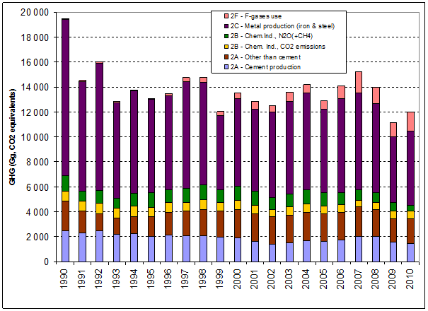
Category 2A (Mineral processes) includes practically only emissions of CO₂, similarly to category 2C (Metal production). CO₂ emissions from the chemical industry are produced by ammonia production, while the production of nitric acid is a source of N₂O emissions. CH₄ emissions from the Industrial processes sector are not significant. Emissions from the use of F-gases (category 2F) are classified in greater detail in the following figure.

Fig. 4‑2 HFC, PFC and SF₆ emissions trends from industrial processes (sector 2F), in 1990 – 2010 [Gg]

4.2 Mineral Products (2A)

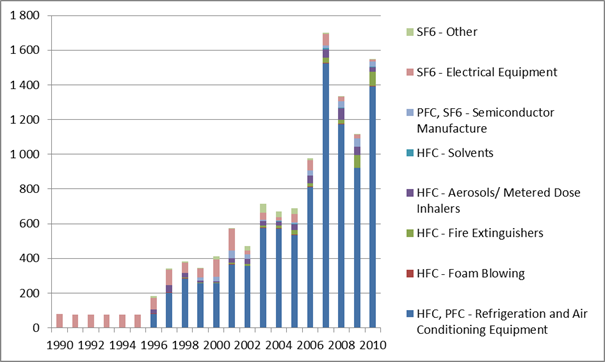
This category describes GHG emissions from the non-fuel emissions from cement and lime production, limestone and dolomite use, glass and ceramics production.

4.2.1 Cement production (2A1)

CO₂ emissions from cement production have decreased since 1990 having the lowest value in 2002. The decrease in the emissions during 1990’s was caused by the transition from planed economy to market economy. This led to decrease in industrial production and also emissions. Since 2003, the cement production began to recover and production increased. Decrease in emissions since 2008 was caused by the economic crisis and related construction constraints.

4.2.1.1 Source category description

Cement production is one of the traditional anthropogenic sources of carbon dioxide included in inventories; however, its importance is incomparably smaller than the total combustion of fossil fuels. Process-related CO₂ is emitted during the production of clinker (calcination process) when calcium carbonate (CaCO₃) is heated in a cement kiln up to temperatures of about 1 300 °C. During this process, calcium carbonate is converted into lime (CaO - calcium oxide) and carbon dioxide. CO₂ emissions from combustion processes taking place in the cement industry (especially heating of rotary kilns) have been reported in IPCC category 1A2f. Limestone (and dolomite) contains also small amount of magnesium carbonate (MgCO₃) and fossil carbon (C), which will also calcinate or oxidize in the process causing CO₂ emissions.

4.2.1.2 Methodological Issues

CO₂ emissions from 2A1 Cement production can be calculated according to the 2000 GPG from the production of cement (Tier 1) or clinker (Tier 2). New IPCC Guidelines (IPCC, 2006) describes a new approach based on direct data from individual operators of cement kilns (Tier 3). Since 2006 submission methodology equal to the Tier 3 has been employed. CO₂ emissions are based on data submitted by the cement kiln operators for preparation and standard operation of the EU ETS system, which includes all the cement kilns in Czech Republic. Information from individual kilns is reported to the competent authority. This data covers years 1990, 1996, 1998 - 2002 and 2005 - 2010. For other years the EF was extrapolated.

The methodology used for CO₂ emissions must be in accordance with national legislation (Vyhláška 12/2009 o stanovení postupu zjišťování, vykazování a ověřování množství emisí skleníkových plynů / Decree 12/2009 establishing a procedure for identifying, reporting and verifying emissions of greenhouse gases) and the EU legislation (Commission Decision of 18 July 2007 establishing guidelines for the monitoring and reporting of greenhouse gas emissions pursuant to Directive 2003/87/EC of the European Parliament and of the Council). The total reported CO₂ emissions from all (5) Czech installations are above 50 kt per year. Two of them reported emissions above 500 kt per year. In all cases, limestone/cement flow is the key parameter, which has the greatest impact on the total emissions from the installation. The content of calcium/magnesium oxide (CaO/MgO) and composition of the limestone and dolomite are measured and independently verified. These parameters are used for calculation of the CO₂ emissions and, therefore, substantial attention is devoted to their determination.

All operating cement plants in the Czech Republic are equipped with dust control technology and the dust is then recycled to the kiln. Only in one cement plant is a small part of the CKD discarded, for technical reasons. Use of dolomite or amount of magnesium carbonate in the raw material, as well as fissile carbon (C) content is known, all above mentioned variables are used for emissions estimates in the EU ETS system. For reasons of confidentiality, it is not possible to make public available all above mentioned data, but only total emission estimates.

Data on cement clinker production is published by the Czech Cement Association (CCA) (CCA, 2010), which associates all Czech cement producers. Clinker production data together with extrapolated EF was used for years without direct data from cement kiln operators. IEF, which is calculated based on CO₂ emissions and clinker production, varies from 0.5267 to 0.5534 t CO₂ / t clinker.

4.2.1.3 Uncertainty and time consistency

All uncertainty estimates of activity data and emission factors have so far been based on expert judgment (see Tab.1‑3, Tab.1‑4 and Tab.1‑5 in Chapter 1.7 on page 47).

Time series consistency is ensured as the above mentioned methodology are employed identically across the whole reporting period from the base year 1990 to 2010.

4.2.1.4 Source-specific QA/QC and verification

General QA/QC procedures and various source specific approaches are used for QA/QC:

· Inter-annual changes of IEF are analyzed.

The EU ETS emissions reports from individual installations are verified by independent verifiers.

Total emissions generated as the sum of emissions from non-combustion processes reported by individual cement kiln operators to the competent authority are compared with the data provided by the Czech Cement Association. Discrepancies are discussed.

4.2.1.5 Source-specific recalculations

No recalculations are applicable for this year.

4.2.1.6 Source-specific planned improvements

It is planed to process all available information about uncertainty form the EU ETS and provide category and national specific uncertainty assessment.

4.2.2 Lime production (2A2)

CO₂ emissions from lime production have decreased considerably since 1990 and were lowest in 2009 (625 Gg CO₂). The decrease in emissions between 1990 and 1991 was caused by the transition from a planned economy to a market economy and closing of lime kilns, together with a decrease in industrial production. Since then, lime production has varied slightly around 1 100 kt/year, except for 2009, when production dropped to a minimum for the whole period of 853 kt. Lime production has reached 915 kt in 2010.

4.2.2.1 Source category description

CO₂ in this category is emitted during the calcination step. Calcium carbonate (CaCO₃) in limestone and calcium / magnesium carbonates in dolomite rock (CaCO₃•MgCO₃) are decomposed to CO₂ and quicklime (CaO) or dolomite quicklime (CaO•MgO), respectively.

4.2.2.2 Methodological Issues

Emissions from lime production were calculated in accordance with 2000 GPG. Only CO₂ emissions generated in the process of the calcination step of lime treatment are considered under category 2A2. CO₂ emissions from combustion processes (heating of kilns and furnaces) are reported under category 1A2f. National EF reflects the production of lime and quick lime (0.7884 t CO₂ / t lime) (Vácha, 2004). Furthermore, it is taken into account the average purity (93%) (Vácha, 2004) of lime produced in Czech Republic.

Activity data are based on statistics from the Czech Lime Association (CLA, 2011), which publishes data on pure lime production, so that these data were considered to be more accurate in comparison with data from the Czech Statistical Office, which do not differentiate between lime and hydrated lime.

Tab. 4‑2 Comparison of CO₂ emissions from lime production 2005 – 2010shows comparison of CO₂ emissions calculated according to IPCC methodology and process-related emissions reported for EU ETS. ETS data closely corresponds to the IPCC methodology and national circumstances.

Tab. 4‑2 Comparison of CO₂ emissions from lime production 2005 – 2010

	Lime produced [t / year]	Process-specific CO₂ emissions [Gg]
	Lime produced [t / year]	IPCC methodology	EU ETS
2005	1 040	763	738
2006	1 034	758	748
2007	1 083	794	772
2008	1 012	742	717
2009	853	625	596
2010	915	671	646

4.2.2.3 Uncertainty and time consistency

All uncertainty estimates of activity data and emission factors have so far been based on expert judgment (see Tab.1‑3, Tab.1‑4 and Tab.1‑5 in Chapter 1.7 on page 47).

Time series consistency is ensured as the inventory approaches concerned are employed identically across the whole reporting period from the base year 1990 to 2010.

4.2.2.4 Source-specific QA/QC and verification

General QA/QC procedures and various source specific approaches are used for QA/QC:

The reports on EU ETS emissions from the individual installations have been verified by independent verifiers. The methodology used for estimation of CO₂ emissions must be in accordance with the national legislation (Vyhláška 12/2009 o stanovení postupu zjišťování, vykazování a ověřování množství emisí skleníkových plynů / Decree 12/2009 establishing a procedure for identifying, reporting and verifying emissions of greenhouse gases) and the EU legislation (Commission Decision of 18 July 2007 establishing guidelines for the monitoring and reporting of greenhouse gas emissions pursuant to Directive 2003/87/EC of the European Parliament and of the Council).

Emission estimates are compared with the sum of emissions from non-combustion processes reported by individual lime kiln operators to the competent authority and with the data provided by the Czech Lime Association (CLA 2011, Yearbook of the Association). Discrepancy was discussed and preliminary result shows that the value of average purity is probably slightly above-estimated.

4.2.2.5 Source-specific recalculations

No recalculations are applicable for this year.

4.2.2.6 Source-specific planned improvements

It is planed to process all available information about uncertainty form the EU ETS and provide category and national specific uncertainty assessment.

4.2.3 Limestone and Dolomite Use (2A3)

Category 2A3 Limestone and Dolomite Use includes emissions from sulphur removal using limestone and emissions from limestone and dolomite use in sintering plants. Emissions from sulphur removal have increased since 1996, when the first sulphur-removal unit came into operation. All Czech thermal power plants have been equipped with sulphur-removal units since 1999. Since 1999, these emissions have varied between 0.5 and 0.6 Mt CO₂ according to electricity production from thermal (brown coal) power plants. Emissions from limestone and dolomite use in sintering plants have fluctuated and were influenced by the transition from a planned economy to a market economy, and restructuring and modernization of the iron and steel industry. The decrease in emissions in 2008 and 2009 was caused by the economic crisis. In 2010 a slight improvement in the economy followed by an increase in emissions was observed.

4.2.3.1 Source category description

From the chemical standpoint, sulphur removal from combustion products in coal combustion, using limestone, is a related source of CO₂ emissions, although it is not of great importance. Here, it holds that one mole of SO₂ removed releases one mole of CO₂without regard to the sulphur-removal technology employed and the stoichiometric excess. Limestone and dolomite are added to sinter where they are calcined, the products subsequently acting as slag formers in blast furnaces.

Emissions from limestone and dolomite which are used for cement production are reported under cement production, similarly to lime and glass production. There is no other known production or process which uses limestone and/or dolomite and produces CO₂ emissions in the CR.

4.2.3.2 Methodological Issues

CO₂ emissions from sulphur removal were calculated from coal consumption for electricity production, the sulphur content and the effectiveness of sulphur removal units between 1996, when the first sulphur removal units came into operation, and 2005. In 2005, these data were verified by comparison with data from the individual power plants, which were collected for EU ETS preparation and which cover the years 1999 – 2005. The EU ETS data form has been used since 2006. The methodology used for estimation of the CO₂ emissions must be in accordance with the national legislation (Vyhláška 12/2009 o stanovení postupu zjišťování, vykazování a ověřování množství emisí skleníkových plynů / Decree 12/2009 establishing a procedure for identifying, reporting and verifying emissions of greenhouse gases) and the EU legislation (Commission Decision of 18 July 2007 establishing guidelines for the monitoring and reporting of greenhouse gas emissions pursuant to Directive 2003/87/EC of the European Parliament and of the Council). Fig. 4‑3 shows comparison of the two methodologies. Tab. 4‑3 lists data for this category.

Emissions from limestone and dolomite use in sintering plants were new source, in 2006 submission, which was identified in the process of preparation of the EU Emission Trading Scheme. Only 2 sintering plants have existed in the CR in recent times. CO₂ emissions from this category are calculated on the basis of data from statistics (The Steel Federation, Inc - production of agglomerate / sinter) and the EF value, which was derived from EU ETS CO₂ emission data based on the limestone and dolomite compositions and consumptions (0.08 t CO₂ / t sinter). Tab 4.3 lists data for this category.

In the CRF tables emissions and activity data for sulphur removal with limestone and emissions from limestone and dolomite use in sintering plants are reported together in the category 2A3 Limestone and Dolomite Use.

Tab. 4‑3 CO₂ emissions from Limestone and Dolomite Use in desulphurization unit, sinter plant, in 1990 – 2010 [Gg]

	CO₂ emissions from desulfurization	CO₂ emissions from sinter plant		CO₂ emissions from desulfurization	CO₂ emissions from sinter plant
1990	NO	678	2001	551	482
1991	NO	605	2002	551	492
1992	NO	283	2003	560	473
1993	NO	251	2004	551	494
1994	NO	291	2005	589	467
1995	NO	519	2006	587	483
1996	76	587	2007	614	492
1997	241	510	2008	607	411
1998	417	492	2009	600	345
1999	537	438	2010	651	370
2000	540	468

4.2.3.3 Uncertainty and time consistency

All uncertainty estimates of activity data and emission factors have so far been based on expert judgment (see Tab.1‑3, Tab.1‑4 and Tab.1‑5 in Chapter 1.7 on page 47).

Time series consistency is ensured for the limestone and dolomite use in sintering plants as the inventory approaches concerned are employed identically across the whole reporting period from the base year 1990 to 2010. Time series for sulphur removal with limestone is not fully consistent as the methodology was changed. The Fig. 4‑3 shows differences between estimates based on coal consumption for electricity production, sulphur content and the effectiveness of sulphur removal and estimates provided for EU ETS.

Fig. 4‑3 Emission estimates comparison for Limestone and Dolomite Use in desulphurization unit, in 1990 – 2010 [Gg]

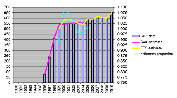
4.2.3.4 Source-specific QA/QC and verification

In the limestone and dolomite use category general QA/QC procedures are used.

4.2.3.5 Source-specific recalculations

No recalculations are applicable for this year.

4.2.3.6 Source-specific planned improvements

It is planed to process all available information about uncertainty form the EU ETS and provide category and national specific uncertainty assessment.

4.2.4 Soda Ash Production and Use (2A4)

4.2.4.1 Source category description

A CO₂ emissions from Soda Ash Production and Use (2A4) category come only from soda ash use. Soda ash is not produced in the CR. Except for the Glass production category, soda ash is used in only one other installation. CO₂ emissions from this category are small and insignificant (approximately 0.4 Gg CO₂) compared to the other categories.

4.2.4.2 Methodological Issues

For each mole of soda ash use, one mole of CO₂ is emitted, so that the mass of CO₂ emitted from the use of soda ash can be estimated from a consideration of the consumption data and the stoichiometry of the chemical process.

The data about the amount and purity of the soda ash used were obtained directly from the installation operator.

4.2.4.3 Uncertainty and time consistency

All the uncertainty estimates related to the activity data and emission factors have so far been based on expert judgment (see Tab.1‑3, Tab.1‑4 and Tab.1‑5 in Chapter 1.7 on page 47).

Time series consistency is ensured as the inventory approaches concerned are employed identically across the whole reporting period from the base year of 2001, when the use of soda started, to 2010.

4.2.4.4 Source-specific QA/QC and verification

General QA/QC procedures are used in the 2A4 Soda Ash Use and Production category.

4.2.4.5 Source-specific recalculations

No recalculations are applicable for this year.

4.2.4.6 Source-specific planned improvements

There are no plans concerning this category.

4.2.5 Other (2A7)

The 2A7 Other category summarizes emissions from Glass Production (2A7.1 – CO₂) and from Brick and Ceramics Production (2A7.2 – CO₂ and CH₄). CO₂ emissions from 2A7.1 Glass production equalled 143 Gg in 2010. Emissions (CO₂ and CH₄) from Brick and Ceramics Production (2A7.2) amounted to 123 kt CO₂ eq. in 2010.

4.2.5.1 Source category description

CO₂ emissions from Glass Production (2A7.1) are derived particularly from the decomposition of alkaline carbonates added to glass-making sand. CO₂ and CH₄ emissions from Brick and Ceramics Production, are derived particularly from the decomposition of alkaline carbonates, fossil and biogenic carbon based substances included in the raw materials.

4.2.5.2 Methodological Issues

The emission factor value of 0.14 t CO₂ / t glass was taken from the new version of the guidebook (EMEP / CORINAIR Atmospheric Emission Inventory Guidebook, 1999). Activity data are collected and published by the Association of the Glass and Ceramic Industry of the Czech Republic.

Emissions from 2A7.2 Brick and Ceramics Production are derived particularly from the decomposition of alkaline carbonates fossil and biogenic carbon based substances included in the raw materials. The EF value was derived from individual installation data collected for EU ETS (emissions) and from CzSO (production). The calculation is based on the total production of ceramic products (fine ceramics, tiles, roofing tiles, and bricks) and the EF value.

4.2.5.3 Uncertainty and time consistency

All uncertainty estimates of activity data and emission factors have so far been based on expert judgment (see Tab.1‑3, Tab.1‑4 and Tab.1‑5 in Chapter 1.7 on page 47).

Time series consistency is ensured as the inventory approaches concerned are employed identically across the whole reporting period from the base year 1990 to 2010.

4.2.5.4 Source-specific QA/QC and verification

In the 2A7 Other category general QA/QC procedures are used.

4.2.5.5 Source-specific recalculations

No recalculations are applicable for this year.

4.2.5.6 Source-specific planned improvements

It is planned to process all the available information about uncertainty from the EU ETS and to provide category and national specific uncertainty assessments. Also it is planned to verify emission estimates with data from the EU ETS system and other available sources.

4.3 Chemical Industry (2B)

Of the categories of sources classified under the Chemical industry (2B), categories 1B1, 1B2 and 1B5 are relevant for the Czech Republic, where adipic acid (1B3) and carbides (1B4) are not produced here.

4.3.1 Ammonia production (2B1)

The production of ammonia constitutes an important source of CO₂ derived from non-energy use of fuels in the chemical industry. CO₂ emissions from ammonia production in 2010 equalled 617.8 Gg of CO₂, corresponding to approx. 0.5% of total greenhouse gas emissions without LULUCF. These emissions decreased by 23% compared to 1990; however, emissions up to 2010 are almost constant, with slight fluctuations. Ammonia production (CO₂ emissions) was not identified as a key category this year (in contrast to some previous years). However, it remains just under the threshold value in the determination by level assessment.

4.3.1.1 Source category description

Industrial ammonia production is based on the catalytic reaction between nitrogen and hydrogen: N₂ + 3H₂ = 2NH₃

Nitrogen is obtained by cryogenic rectification of air and hydrogen is prepared using starting materials containing bonded carbon (such as, e.g., natural gas, residual oil, heating oil, etc.). Carbon dioxide is generated in the preparation of these starting materials.

In the Czech Republic, hydrogen for ammonia production is derived from residual oil from petroleum refining, which undergoes partial oxidation in the presence of water vapour. In order to increase the hydrogen production, the second step involves conversion of carbon monoxide, which is formed by partial oxidation, in addition to carbon dioxide and hydrogen. The final products of this two-step process are hydrogen and carbon dioxide. The production technology has practically not changed since 1990.

4.3.1.2 Methodological Issues

Emissions are calculated from the corresponding amount of ammonia produced, using the technologically-specific emission factor 2.40 Gg CO₂ / Gg NH₃ (Markvart and Bernauer, 2005 - 2010). This emission factor was derived from the relevant technical literature - Ullman’s Encyclopedia (Wiley, 2005) corresponding to the ammonia production employed in the Czech Republic, including information required for deriving the carbon dioxide emission factor: 56.25 t NH₃ are produced from 44 t of residual oil containing 84.6% C. Simple stoichiometric calculation yields the value of the emission factor EF CO₂ = 2.402 t CO₂/t NH₃. This emission factor includes the efficiency of the conversion of carbon contained in the starting material to carbon dioxide, equal to 99% (i.e. an oxidation factor of 0.99).

A potential uncertainty in the emission factor for ammonia would not influence the total sum of CO₂ emissions because a corresponding amount of oil is not considered in the energy sector. The relevant activity data and corresponding emissions are given in Tab. 4‑4 Activity data and CO₂ emissions from ammonia production in 1990 – 2010

Tab. 4‑4 Activity data and CO₂ emissions from ammonia production in 1990 – 2010

Year	1990	1991	1992	1993	1994	1995	1996	1997
Residual fuel oil used for NH₃ product., [TJ]	11113	10770	11104	10383	11593	10235	11015	10095
Ammonia produced, [kt]	335.9	325.5	335.6	313.8	350.4	309.3	332.9	305.1
CO₂ from 2B1, [Gg]	806.8	781.9	806.1	753.8	841.6	743.0	799.7	732.9

Year	1998	1999	2000	2001	2002	2003	2004	2005
Residual fuel oil used for NH₃ product., [TJ]	10407	8864	10144	8538	7449	9696	9721	8478
Ammonia produced, [kt]	314.5	267.9	306.6	258.0	225.1	293.0	290.8	253.6
CO₂ from 2B1, [Gg]	755.5	643.6	736.5	619.9	540.8	703.9	698.7	609.3

Year	2006	2007	2008	2009	2010
Residual fuel oil used for NH₃ product., [TJ]	8086	7575	8487	8739	8510
Ammonia produced, [kt]	241.9	226.6	256.5	264.1	257.2
CO₂ from 2B1, [Gg]	581.1	544.4	616.3	634.4	617.8

4.3.1.3 Uncertainty and time consistency

All uncertainty estimates of activity data and emission factors have so far been based on expert judgment (see Tab.1‑3, Tab.1‑4 and Tab.1‑5 in Chapter 1.7 on page 47).

Time series consistency is ensured as the above mentioned methodology are employed identically across the whole reporting period from the base year 1990 to 2010.

4.3.1.4 Source-specific QA/QC and verification

The sector-specific QA/QC plan follows from the overall plan described in Chapter 1. Attention was focused on identifying gaps and imperfections using the reporting software (CRF Reporter), specifically by observing trends in figures and by checking IEFs. Attention was also focused on checking sources from inter-sector boundaries (Energy, Industry) that they are neither omitted nor counted twice. Therefore CO₂ emissions from residual oil used for ammonia production are not taken into account in Energy sector. This part of QA/QC procedure is carried out in cooperation with experts from KONEKO.

4.3.1.5 Source-specific recalculations

No recalculations were employed in this category in this submission.

4.3.1.6 Source-specific planned improvements

It is planed to continue improvement of the uncertainty data.

4.3.2 Nitric acid production (2B2)

The production of nitric acid constitutes one of the most important sources of N₂O in the chemical industry. N₂O emissions from production of nitric acid in 2010 equalled 1.21 Gg N₂O, corresponding to approx. 0.4 % of total greenhouse gas emissions without LULUCF. These emissions have decreased by 67% compared to 1990; the substantial decrease in recent years has been a consequence of the gradual introduction of mitigation technology and improving its effectiveness. In 2010, the production of nitric acid (N₂O emissions) was identified as a key category by trend assessment. In former years, when N₂O emissions reached greater values, this category was identified as a key source by level assessment.

4.3.2.1 Source category description

The production of nitric acid is one of the traditional production processes in the Czech Republic. It is produced in three factories, where one of them manufactures more than 60% of the total amount. Nitric acid is produced by the classical method by high-temperature catalytic oxidation of ammonia and subsequent absorption of nitrogen oxides in water. Nitrous (dinitrogen) oxide is formed in the production of the acid as an unwanted side product.

The production process is performed in the Czech Republic at three pressure levels (at atmospheric pressure, slightly elevated pressure (approx. 0.4 MPa) and at elevated pressure (0.7 - 0.8 MPa). While production processes prior to 2003 mostly progressed at atmospheric pressure and only to a lesser degree at medium elevated pressure, the process at elevated pressure had predominated since 2004.

All the production processes in the Czech Republic are equipped with technologies for removal of nitrogen oxides, NO_x, based on selective or non-selective catalytic reduction. Non-selective catalytic reduction also makes a substantial contribution to removal of N₂O. Since 2004, technology to reduce N₂O emissions, based on catalytic decomposition of this oxide, has been gradually introduced at units working at elevated pressure. It has been possible to substantially improve the effectiveness of this process in recent years.

4.3.2.2 Methodological Issues

Nitrous oxide emissions from 2B2 Nitric Acid Production are generated as a by-product in the catalytic process of oxidation of ammonia. It follows from domestic studies (Markvart and Bernauer, 1999, 2000, 2003), describing conditions prior to 2004, that the resulting emission factor depends on the technology employed: higher emission factor values are usually given for processes carried out at normal pressure, while lower values are usually given for medium-pressure processes. Two types of processes were carried out in this country before 2004, at pressures of 0.1 MPa and 0.4 MPa. The amount of nitrous oxide in the exit gases is also affected by the type of process employed to remove nitrogen oxides, NO_x (i.e. NO and NO₂). In this country, the process of Selective Catalytic Reduction (SCR) is mostly used, which slightly increases the amount of N₂O, and also to a certain degree Non-Selective Catalytic Reduction (NSCR), which also removes N₂O to a considerable degree.

Studies (Markvart and Bernauer, 2000, 2003) recommend the following emission factors for various types of production technology and removal processes that are given in Tab. 4‑5. The emission factors for the basic process (without DENOX technology) are in accord with the principles given in the above-cited IPCC methodology. The effect of the NO_x removal technology on the emission factor for N₂O was evaluated on the basis of the balance calculations presented in studies (Markvart and Bernauer, 2000, 2003).

Tab. 4‑5 Emission factors for N₂O recommended by (Markvart and Bernauer, 2000) for 1990 - 2003

Pressure in HNO₃production	0.1 MPa			0.4 MPa
Technology DENOX	--	SCR	NSCR	--	SCR	NSCR
Emission factors N₂O [kg N₂O / t HNO₃]	9.05	9.20	1.80	5.43	5.58	1.09

Collection of activity data for HNO₃production is more difficult than for cement production because of the present legislation, which complicates the releasing of statistical data on manufactured products where the number of producers is smaller than (or equal to) three. Therefore, it was necessary to obtain them by questioning all three producers in the Czech Republic, see (Markvart and Bernauer, 2000, 2003, 2004).

During 2003, conditions changed substantially as a result of the installation of new technologies operating under higher pressure of 0.7 MPa. At the same time, some older units operating under atmospheric pressure of 0.1 MPa were phased out. These changes in technology were monitored in the study of Markvart and Bernauer (Markvart and Bernauer, 2005). This study presents a slightly modified table of N₂O emission factors, while those for new technologies were obtained from a set of continuous emission measurements lasting several months. Other values are based on several discrete measurements. A table of these technology-specific emissions factors is given below.

Tab. 4‑6 Emission factors for N₂O recommended by Markvart and Bernauer, for 2004 and thereafter

Pressure	0.1 MPa	0.4 MPa	0.4 MPa	0.7 MPa
DENOX process	SCR	SCR	NSCR	SCR
EF, kg N₂O / t HNO₃ (100 %)	9.05	4.9	1.09	7.8 ^a)

^a)EF without N₂O mitigation. Cases of N₂O mitigation in 2005 -2008 are shown in Tab. 4‑7

In the last quarter of 2005, a new N₂O mitigation unit based on catalytic decomposition of N₂O was experimentally installed for 0.7 MPa technology, and became the most important such unit in the Czech Republic. As a consequence of this technology, the relevant EF decreased from 7.8 to 4.68 kg N₂O/t HNO₃ (100 %). Therefore, the mean value in 2005 for the 0.7 MPa technology was equal to 7.02 kg N₂O/t HNO₃ (100 %), (Markvart and Bernauer, 2006)

In 2006 - 2010, the mitigation unit described above was utilized in a more effective way, see (Markvart and Bernauer, 2007 - 2011). The decrease in the emission factor for 0.7 MPa technology as a result of installation of the N₂O mitigation unit and gradual improvement of the effectiveness is given in Tab. 4‑7.

Two high temperature N₂O decomposition catalytic systems were used in the above-mentioned high pressure nitric acid technology (0.7 MPa) in 2009; these systems were more efficient in comparison with the catalytic systems used in previous years. The first system consisting of Raschig rings provided by Heraeus was used in the January-June 2009 period and the measured EF N₂O was 3.10 kg N₂O/ t HNO₃ (100 %); in the July-November 2009 period, EF N₂O was 3.30 kg N₂O/ t HNO₃ (100 %). The second system consisting of high temperature N₂O decomposition catalyst developed by YARA company, decreased EF N₂O in the November-December 2009 period to the value 0.95 kg N₂O/ t HNO₃ (100 %) in a high-pressure nitric plant. The catalytic activity of the high temperature decomposition system has decreased slightly due to both increasing selectivity of the Pt-Rh ammonia oxidation catalyst towards N₂O and slow deactivation of the N₂O decomposition catalyst. Thus, the mean value of EF N₂O for this high pressure nitric acid technology in 2009 was assessed at a value of 2.85 kg N₂O/ t HNO₃ (100 %) (Tab. 4‑7).

The most efficient decomposition catalyst provided by YARA was used in this high pressure nitric acid technology during whole year of 2010. It is expected that, if high temperature N₂O decomposition catalyst (i.e. YARA catalyst) is employed, the EF N₂O could be approximately close to 1.3 kg N₂O/ t HNO₃ (100 %).

Tab. 4‑7 Decrease in the emission factor for 0.7 MPa technology due to installation of the N₂O mitigation unit

Year	2004 ^a)	2005	2006	2007	2008	2009	2010
EF, kg N₂O / t HNO₃ (100 %)	7.8	7.02	5.94	4.37	4.82	2.85	1.29
Effectiveness of mitigation, %	-	10	23.9	43.9	38.2	63.4	83.4

^a)EF without N₂O mitigation.

The emission factors used in the Czech Republic are compared with the EFs presented in the IPCC methodology (IPCC, 2000) in the Tab. 4‑8.

Tab. 4‑9 gives the N₂O emissions from production of nitric acid, including the production values.

Tab. 4‑8 Comparison of emission factors for N₂O from HNO3 production

Production process

N₂O Emission factor (kg N₂O/t 100% HNO3)

Reference

Canada

Plants without NSCR

Plants with NSCR

8.5

(IPCC, 2000)

USA

Plants without NSCR

Plants with NSCR

9.5

(IPCC, 2000)

Norway

Process-integrated N₂O destruction

Atmospheric pressure plant

Medium pressure plant

4–5

6–7.5

(IPCC, 2000)

Other countries

Dual-pressure plant (European design)

Older plants (pre-1975), without NSCR

8–10

10–19

(IPCC, 2000)

Czech Republic

Atmospheric pressure plants

Medium pressure plants with SCR

Medium pressure plants with NSCR

High pressure plants SCR (no N₂O decomposition)

High pressure plants SCR (with N₂O decomposition)

9.05

4.9

1.09

7.8

4.82 – 1.29

(Markvart and Bernauer, 2009, 2010)

Tab. 4‑9 Emission trends for HNO3 production and N₂O emissions

	Production of HNO₃, *[Gg HNO₃ (100 %)]*	*Emissions of N₂O [Gg N₂O]* from HNO₃production**
1990	530.0	3.63
1991	349.6	2.37
1992	439.4	2.98
1993	335.9	2.27
1994	439.8	2.94
1995	498.3	3.37
1996	484.8	3.06
1997	483.1	3.33
1998	532.5	3.59
1999	455.0	2.95
2000	505.0	3.36
2001	505.1	3.32
2002	437.1	2.87
2003	500.6	2.86
2004	533.7	3.27
2005	532.2	3.09
2006	543.1	2.76
2007	554.2	2.28
2008	507.0	2.14
2009	505.2	1.63
2010	441.7	1.21

4.3.2.3 Uncertainty and time consistency

All uncertainty estimates for the activity data and emission factors have so far been based on expert judgment (see Tab.1‑3, Tab.1‑4 and Tab.1‑5 in Chapter 1.7 on page 47). Their improvement is ongoing and some uncertainty values for HNO₃ production have been recently revised and used in the two last submissions: uncertainty in activity data was lowered from 10 % to 5 % and uncertainty of the mean N₂O EF was lowered from 25 % to 20 %.

Time series consistency is ensured as inventory approaches concerned are employed identically across the whole reporting period from the base year of 1990 to 2010.

4.3.2.4 QA/QC and verification

The sector-specific QA/QC plan follows from the overall plan described in Chapter 1. Attention is focused on identifying gaps and imperfections using the reporting software (CRF Reporter), specifically by observing trends in figures and by checking IEFs.

According to the QA/QC plan, data and calculations are provided by the external consultants (M. Markvart and B. Bernauer) are checked by the experts from CHMI and vice versa.

Technology-specific methods for N₂O emission estimates have been improved by incorporating direct emission measurements, especially for new technology (0.7 MPa), which is now predominant in the Czech Republic.

4.3.2.5 Recalculations

No recalculations in the 2B2 category were employed in this submission.

4.3.2.6 Source-specific planned improvements

It is planed to continue improvement of the uncertainty data.

4.3.3 Other (2B5)

4.3.3.1 Source category description

This category includes methane emissions from the production of carbon black, ethylene, dichloroethylene, styrene, methanol and N₂O emissions from the production of caprolactam. These are all less important sources.

4.3.3.2 Methodological issues

Default emissions from the IPCC methodology (IPCC, 1997) are employed to determine methane emissions from the production of carbon black, ethylene, dichloroethylene, styrene and methanol.

CH₄ emissions from the production of carbon black

The nominal capacity is currently 300 t p.a. Exact information on activity data is not available for the individual years; thus, the data were taken as the expert estimates mentioned in the study (Markvart and Bernauer, 2011), taking into account the increase in carbon black consumption in the rubber industry:

1990-2000 200 t carbon black p.a.

2001-2005 250 t carbon black p.a.

2006-2010 300 t carbon black p.a.

The emission factor taken from the IPCC method equals 0.11 kt CH₄/kt carbon black, so that the highest value of methane emissions over the past few years is practically insignificant (0.0033 Gg).

CH₄ emissions from the production of ethylene

Reliable data for the production of ethylene are available from CzSO. The IPCC methodology yields a value of 0.001 kt/kt for the default emission factor for methane. In 1990 – 2010, methane emissions varied between 0.3 and 0.5 Gg CH₄ (emissions equalled 0.455 Gg CH₄ in 2010).

CH₄ emissions from the production of dichloroethylene

While CzSO does not publish information on the amount of dichloroethylene produced, it does give data on the amount of PVC produced. The study (Markvart and Bernauer, 2011) recommends multiplying the amount of PVC produced by a coefficient of 1.23 derived from the stoichiometry. The IPCC methodology yields a value of 0.0004 kt/kt for the default emission factor for methane. Because of the low emission factor value, the values of methane emissions varied in 1990 – 2010 between 0.04 and 0.06 Gg CH₄ – and this is thus a not very significant value. Emissions equalled 0.054 Gg CH₄ in 2010.

CH₄ emissions from the production of styrene

Because of the growing consumption of polystyrene, the production of styrene has gradually increased since 1990. CzSO also does not publish any information on the production of styrene. Thus, the necessary activity data were estimated on the basis of production capacities:

1990-1998 70 kt styrene p.a.

1999 80 kt styrene p.a.

2000-2003 110 kt styrene p.a.

2004 140 kt styrene p.a.

2005-2009 150 kt styrene p.a.

from 2010 170 kt styrene p.a.

These estimates of data on the amount of styrene produced, mentioned in the study (Markvart and Bernauer, 2011), are based on the data given in the article (Dvořák and Novák, 2010). The emission factor taken from the IPCC method equals 0.004 kt CH₄/kt styrene. In 1990 – 2010, methane emissions varied between 0.3 and 0.7 Gg CH₄ (emissions equalled 0.68 Gg CH₄ in 2010).

Methanol is not produced in the Czech Republic and thus the symbol “NO” applies to the entire time period from 1990.

Production of caprolactam

As mentioned in the references (Markvart and Bernauer, 2004 – 2011), there is only one caprolactam production plant in the Czech Republic; this is not a very important source of N₂O emissions. CzSO does not monitor production data on the production of caprolactam; however, the series of studies by Markvart and Bernauer (Markvart and Bernauer, 2004 – 2011), based on a study in the production factory, yields an approximate value of 0.27 Gg N₂O for the period to 2005 and, following 2006, a value of 0.305 Gg N₂O, based on increased production capacity. More exact data should be available in the coming years, when the N₂O emissions from the production of caprolactam will be continuously measured from 2012 as a consequence of inclusion of the production in the emission trading scheme (EU ETS) and thus recording in the relevant register.

4.3.3.3 Uncertainty and time consistency

In relation to the relatively insignificant greenhouse gas emissions from category 2B5, uncertainties derived from the sources included in this category have no great impact on the overall uncertainty in the determination of GHG emissions in the Czech Republic Thus, it does not matter greatly that the uncertainty in emissions from these sources was determined by an expert estimate; the numerical values are given in Tab.1‑3, Tab.1‑4 and Tab.1‑5 in Chapter 1.7 on page 47.

4.3.3.4 QA/QC and verification

In relation to the relatively unimportant greenhouse gas emissions from category 2B5, only QC, Tier 1 procedures were used, in accordance with the QA/QC plan.

4.3.3.5 Recalculations

In former submissions, CH₄ emissions were reported for the production of carbon black, dichloroethylene and styrene only following 2008 because of the lack of the activity data required for determining emissions. However, the authors of the study (Markvart, Bernauer, 2011) recently managed to obtain the data required for determining CH₄ emissions from 1990 (see the “Methodical Issues” section). The newly determined values (replacing symbol “NE”) must be seen as recalculations. This increase in the completeness of the inventory has resolved the repeated recommendations of the international inspection team over the past years.

4.3.3.6 Source-specific planned improvements

More exact data on N₂O emissions should be available in the coming years, when the N₂O emissions from the production of caprolactam will be continuously measured beginning in 2012 as a consequence of inclusion of the production in the emission trading scheme (EU ETS) and thus recording in the relevant register. No further improvement is planned for methane emissions in this category.

4.4 Metal Production (2C)

4.4.1 Source category description

This category includes mainly CO₂ emissions from 2C1 Iron and Steel Production. CO₂ emissions from iron and steel are identified as a key category (by both level and trend assessments). A small amount of CH₄ is also emitted.

Ferro-alloys were manufactured in limited amounts in a small production unit in the Czech Republic; this process could constitute an unsubstantial source of CO₂ emissions. Unfortunately, CzSO does not monitor any data on this production process. Investigation revealed one smaller production plant, which reported that aluminium was used as a reducing agent; this did not lead to CO₂ emissions. In 2009 this production was stopped.

Iron is produced in the Czech Republic in two large metallurgical works located in the cities of Ostrava and Třinec in the Moravian-Silesian Region, in the north-eastern part of the Czech Republic. Both these metallurgical works employ blast furnaces and also lines for the production of steel, coking furnaces and other supplementary technical units. Another large steel plant is located immediately next to the metallurgical works in Ostrava, taking raw iron (in the liquid state) from the nearby blast furnaces (located in the area of the Ostrava metallurgical works).

4.4.2 Methodological Issues

CO₂ emissions were determined for category 2C1 using a procedure corresponding to Tier 1 of the Good Practice Guidance for 2C1. This calculation was based on the amount of coke consumed in blast furnaces. The calculation was carried out using NCV = 27.87 MJ/kg in 2010 (NCV interval for period 1990 - 2010 is (27.9 - 28.8 MJ/kg) and using the carbon emission factor for coke, 29.5 t C / TJ, which is the IPCC default value (IPCC, 1997). As the final products in metallurgical processes are mostly steel and iron with very low carbon contents, the relevant correction for the amount of carbon remaining in the steel or iron was taken into account by using factor 0.98, i.e. the same factor that is standardly used for combustion of solid fuels (the oxidation factor). The major part of CO₂ emissions calculated in this manner is, in reality, emitted in the form of the products of combustion of blast-furnace gas occurring mainly in metallurgical plants, while a smaller part is emitted from heat treatment of pig iron during its transformation to steel.

The relevant activity data and corresponding emissions are given in Tab. 4‑10 Activity data and CO₂ emissions from iron and steel in 1990 - 2010.

Tab. 4‑10 Activity data and CO₂ emissions from iron and steel in 1990 - 2010

Year	1990	1991	1992	1993	1994	1995	1996	1997
Coke consumed in blast furnaces, [kt]	4 222	2 959	3 447	2 582	2 724	2 857	2 701	2 846
CO₂ from 2C1, [Gg]	12 533	8 781	10 230	7 690	8 231	7 523	7 861	8 520

Year	1998	1999	2000	2001	2002	2003	2004	2005
Coke consumed in blast furnaces, [kt]	2 750	1 941	2 327	2 175	2 252	2 459	2 628	2 260
CO₂ from 2C1, [Gg]	8 233	5 945	7 027	6 625	6 861	7 484	7 798	6 687

Year	2006	2007	2008	2009	2010
Coke consumed in blast furnaces, [kt]	2 480	2 570	2 366	1 742	2 004
CO₂ from 2C1, [Gg]	7 573	7 757	7 151	5 298	5 919

Estimation of CH₄ from metal production is based on the CORINAIR methodology. Metal production emits only 2.3 – 6.0 Gg of methane.

Emissions of methane in 2010 equaled 2.6 Gg, of which 1.3 Gg corresponds to the contribution of methane emissions from coke production. In this case, the relevant activity data correspond to the amount of coke produced from the Energy Balances of the CR are given in CRF Tables. In contrast, the activity data used for calculation of CO₂ emissions, correspond to the amount of coke consumed in blast furnaces. These data were determined from the CzSO material “Energy intensity of manufacture of selected products". It should be pointed out that these two series are not completely identical (e.g. part of the coke produced is used for other purposes and imported coke can also be used in blast furnaces).

Emission estimates of precursors for the relevant subcategories have been transferred from NFR to CRF, as described in previous chapters.

4.4.3 Uncertainty and time consistency

The uncertainty estimates were based on expert judgment (see Tab.1‑3, Tab.1‑4 and Tab.1‑5 in Chapter 1.7 on page 47). Their improvement is ongoing and is planned for inclusion in the next NIR.

Consistency of the time series is ensured as the inventory approaches concerned are employed identically across the whole reporting period from the base year of 1990 to 2010.

4.4.4 QA/QC and verification

The sector-specific QA/QC plan follows from the overall plan described in Chapter 1. The greatest attention was focused on identifying gaps and imperfections using the new reporting software (CRF Reporter), specifically by observing trends in figures and by checking IEFs. Attention was also focused on checking sources from inter-sector boundaries (Energy, Industry) that they are neither omitted nor counted twice. CO₂ emissions from coke used in blast furnaces are not considered in Energy sector.

Activity data available in the official CzSO materials in relation to QA/QC were independently determined by experts from CHMI and KONEKO and were mutually compared. Experts at CHMI additionally checked most of the calculations carried out by experts at KONEKO and vice versa.

4.4.5 Recalculations

In the 2011 submission, the recalculation for the 2003 - 2008 period was performed for CO₂ emissions from 2C1 (Iron and steel production). Estimation of these emissions in the Czech Republic is based on the amount of coke consumed in blast furnaces. This amount (directly in TJ) was originally taken from the document provided by the Czech Statistical Office (CzSO) “Development of overall and specific consumption of fuels and energy in relation to product”.

For this recalculation, the other official document of CzSO “CzSO (2010): Energy Questionnaire - IEA / Eurostat (CZECH_COAL, CZECH_OIL, CZECH_GAS, CZECH_REN), Prague 2010” was used as a source of data on metallurgical coke consumed in blast furnaces. This approach, which is more consistent with that used for the Energy sector since 2003, was recommended by experts from CzSO because of better accuracy and reliability of coke data. However, differences between the two sources of data are not very substantial: e.g. for 2003, the recalculated CO₂ emission value is 1.2% lower than the original value, for 2008 the recalculated CO₂ emission value is 3.8% lower than the original value and for 2009 the newly estimated CO₂ emission value is 4.4% higher than the value that would be obtained by the older approach.

In the 2012 submission (i.e. in this submission), the above mentioned recalculation was extended for the 1995 – 2002 period. With exception of 1995 and 1998, differences in CO₂ emissions calculated from the two sources are less the 2%. Similarly as in the case of 2011 submission, the present recalculations were also harmonized with recalculations in the sector Energy.

4.4.6 Source-specific planned improvements

It is planned to implement uncertainty assessment. Moreover, application of more advanced Tier 2 methodology for Iron and steel production is planned in the future. At the present time, options are being explored for obtaining the relevant data for this purpose.

4.5 Other Production (2D)

In this sector are reported only indirect GHGs and SO₂ from sectors Pulp and Paper; Food and Drink.

4.6 Production of Halocarbons and SF₆ (2E)

Halocarbons and SF₆are not produced in Czech Republic.

4.7 Consumption of Halocarbons and SF₆ (2F)

4.7.1 Source Category Description

Emissions of F-gases (HFCs, PFCs, SF₆) in the Czech Republic are at a relatively low level due to the absence of large industrial sources of F-gases emissions. As mentioned above, F-gases are not produced in the Czech Republic and therefore there are no fugitive emissions from manufacturing. Additionally, there is no production of other fluorinated gases (CFCs, HCFCs, etc.) that could lead to by-product F-gases emissions and there is no aluminum and magnesium industry in the Czech Republic. F-gases emission in 2009 dropped compared to 2008 as result of finance crisis and lower production in air-conditioning, refrigeration and car industry.

F-gases emissions from national sources are coming only from their consumption in applications as follows:

SF₆ used in electrical equipment,
SF₆ used in sound proof windows production,
SF₆ used in special applications (laboratory),
HFCs, PFCs and SF₆ used in semiconductor manufacturing,
HFCs and PFCs used as refrigerants in refrigeration and air conditioning equipment,
HFCs used as propellants in aerosols,
HFCs used as blowing agents,
HFCs used as extinguishing agents in fixed fire fighting systems.

No official statistics that would allow easy disaggregated reporting and / or use of the highest tiers are currently available in the Czech Republic. All the data are collected based on voluntary cooperation between sectoral experts and private companies.

For source consumption of F-gases, potential emissions increased from 169.4 Gg CO₂eq. in 1995 to 3 915.6 Gg CO₂eq. in 2010. The significant increase compared to 2009 could be explained mainly by the economic recovery and a substantial increase in the use of HFCs. For the source consumption of F-gases, actual emissions increased from 76.1 Gg CO₂eq. in 1995 to 1 549.0 Gg CO₂eq. in 2010. This significant increase could be explained as being mainly due to a substantial increase in the use of HFCs in refrigeration. The marked sharp decrease between 2007 and 2009 is due to a production decrease as a result of the financial crisis. Detailed information about actual and potential emissions is given in Tab. 4‑11 and the CRF Tables.

Tab. 4‑11 HFCs, PFCs and SF₆ potential and actual emissions in 1995 - 2010 [Gg CO₂ eq.]

	Potential				Actual
	HFCs	PFCs	SF₆	Total	HFCs	PFCs	SF₆	Total
1995	2.21	0.35	166.82	169.38	0.73	0.12	75.20	76.06
1996	134.51	4.22	183.07	321.80	101.31	4.11	77.52	182.94
1997	479.44	1.17	180.49	661.10	244.81	0.89	95.48	341.18
1998	577.87	1.17	126.02	705.07	316.56	0.89	64.19	381.63
1999	411.87	2.74	110.90	525.50	267.47	2.55	76.98	347.01
2000	674.32	9.45	206.02	889.79	262.50	8.81	141.92	413.23
2001	1045.13	14.49	223.23	1282.84	393.37	12.35	168.73	574.45
2002	1092.41	17.91	211.85	1322.17	391.29	13.72	67.72	472.73
2003	1343.94	28.64	339.26	1711.84	590.14	24.53	101.25	715.93
2004	1215.00	20.98	208.00	1443.98	600.30	17.33	51.89	669.51
2005	1280.55	13.77	156.88	1451.20	594.21	10.08	85.88	690.17
2006	2573.99	30.33	161.90	2766.21	872.35	22.56	83.07	977.98
2007	3884.78	27.57	133.84	4046.18	1605.85	20.16	75.85	1701.86
2008	3053.38	38.25	85.32	3176.95	1262.45	27.48	47.04	1336.98
2009	2355.90	39.38	132.17	2527.44	1045.67	27.14	49.61	1118.41
2010	3854.62	44.25	16.73	3915.60	1503.36	29.43	16.22	1549.01

4.7.2 General Methodological Issues

Currently, the national F-gases inventory is based on the method of actual emissions. The method of potential emissions is used only as supporting information.

According to the Revised 1996 IPCC Guidelines (IPCC, 1997), potential emissions have been calculated from the consumption of F-gases (sum of domestic production and import minus export and environmentally sound disposal). Due to the relatively short time of use of F-gases, it has been assumed that the disposed amount is relatively small. In 2010, a small amount of destroyed F-gases was reported. The main part of these gases was imported to CR for destruction and did not come from equipment operating in the CR. The potential methodology is the same for all categories of use of F-gases. The actual emissions methodology is specified for each category.

As these substances are not nationally produced, import and export information coming from official customs authorities are of the key importance. Individual F-gases do not have a separate custom codes in the customs tariff list as individual chemical substances. SF₆ is listed as a part of cluster of non-metal halogenides and oxides, HFCs and PFCs are listed as total in the cluster of halogen derivatives of acyclic hydrocarbons. In order to determine the exact amounts of these substances, it is essential to obtain information from the customs statistics and from individual importers and exporters, about (a) the imported and exported amounts and (b) kinds of substances (or their mixtures), (c) the amounts and types of disposed F-gases and also (d) the areas of usage. For the first year, also data about direct import, export, use and destruction were obtained from ISPOP. ISPOP is national system of environmental reporting; all importers, exporters and users of more than a threshold of 100 kg should report information about the type and amount of F-gases used. Because this was the first year of reporting and problems related to the completeness and correctness were expected, similarly as in previous years, all the importers, exporters and users were requested to complete a specific questionnaire on export and import of F-gases and to support the questionnaire by additional information on the quantity, composition and use. More detailed description of the methodology is available under the separate document (Řeháček and Michálek, 2005) which also contents all relevant information for potential and actual emissions calculations. Emissions of F-gases are based on data on import and export of individual chemicals or their mixtures (as bulk), but not on products.

4.7.3 Sector-Specific Methodological Issues

This chapter specifies the actual emissions methodology used for a given sector. In the following chapters, individuals sectors with similar methodology are connected, e.g. a similar approach is used in the foam blowing and sound-proof windows sectors for estimation of actual emissions, and thus the approach is described in one joint chapter. Detailed information on the data and methodology used are included in a special report prepared by the external co-worker Mr. Řeháček in 2011 (Řeháček, 2011).

The most important category in view of actual emissions is Refrigeration and Air Conditioning Equipment, which is responsible for 89.9 % of actual F-gases emissions.

4.7.3.1 Refrigeration and Air Conditioning Equipment

In the CRF Tables, emissions from this category are divided into only two sub-categories: 2IIAF11 Domestic Refrigeration and 2IIAF16 Mobile Air-Conditioning; emissions from other subcategories are also included in these two categories, because of the lack of detailed information. The methodology used in these calculations underestimated real emissions, as information about the lifetimes of products that contain F-gases is not taken into account. The underestimation for 2010 is relatively low, but will be a very important “source” in a few years, e.g. in 2025 it will correspond to additional emissions of approximately 1.5 mil t CO₂ eq.

Emissions from Mobile Air-Conditioning include mainly emissions from the “First-Fill” in three Czech car factories and from the relatively small amount used for servicing old equipment. The calculation was performed using Equation 3.44 from 2000 GPG; recently, it has been assumed that emissions from disposal and destruction are negligible because of the relatively short time of use of F-gases in this sector. This fact is also supported by the information on disposed refrigerants (Řeháček, 2010). The contribution of this sector to total actual F-gases emissions was 28.6 % in 2010. It can be anticipated that emissions from this category will increase in the future.

Emissions from Domestic Refrigeration include emissions from servicing old equipment and emissions from production of new air-conditioning equipment since 2007. The calculation is performed using the Tier 2 top-down approach methodology (Equation 3.40 from 2000 GPG). This sector has the greatest share on the total actual emissions of F-gases, which equalled 61.2 % in 2010.

4.7.3.2 Foam Blowing and Production of Sound-Proof Windows

F-gases were used in the Czech Republic only for producing hard foam. Only HFC-143a was used regularly for foam blowing. HFC-227ea and HFC-245ca were used once for testing purposes. SF₆ is used for production of sound-proof windows. The amount of SF₆ used for production of sound-proof windows has been decreasing since 2003. SF₆ was not used for the first fill of new sound-proof windows and emissions in 2010 come only from stock. Emissions from these different categories are calculated in a similar way. The default methodology and EF described in 2000 GPG are used for sound-proof windows, specifically Equations 3.24 and 3.35. Similar equations are used for foam blowing. The contribution of foam blowing and production of sound-proof windows to total emissions of F-gases equalled 0.2 and 0.2 %, respectively, in 2010.

4.7.3.3 Fire Extinguishers

In this category only PFC emissions are used and reported. Emission from this category is calculated on the basis of GPG 2000. Calculations are based on data about production of new equipment and data about service of old equipment. PFC was not used for the first fill of new equipment; emissions came only from service of old equipment in 2010. The share of this sector in the total actual F-gases emissions was 5.2 % in 2010.

4.7.3.4 Aerosols / Metered Dose Inhalers and Solvents

Emissions from these categories (2F4 Aerosols / Metered Dose Inhalers and 2F5 Solvents) are based on 2000 GPG and Equation 3.35; EF equals 50 %. A small amount of F-gases as solvents was reported in the Czech Republic in 2010. The contribution of these sectors to the total actual F-gas emissions equalled 1.8 and 0.03 %, respectively, in 2010.

4.7.3.5 Semiconductor Manufacture

Actual emissions from this category are calculated on the basis of Tier 1 methodology. Emissions from this category correspond to 1.9 % of the total actual 2010 emissions of F-gases. No data are available for more precise emission calculations and this category is not very important.

4.7.3.6 Electrical Equipment

Emissions from this category are calculated according to 2000 GPG, specifically Equation 3.13, which is called the Tier 3a method. Basic data about new equipment and services can be obtained from the above-mentioned questionnaires. This equipment is produced by only one company and is serviced by several companies. Emissions from this category correspond to 0.8 % of the total actual emissions of F-gases in 2010. The share of this category in the total actual emissions has decreased rapidly since 1995 due to a decrease in the use of SF₆ in this sector and increase in the use of HFCs in refrigeration.

4.7.3.7 Others

This category includes the 2F9 Other / Laboratories category. This category was included in the 2006 submission for the first time and encompasses emissions of SF₆ from laboratory use. The amount of F-gases in 2010 was not identified in this category. Potential and actual emissions are calculated in the same way in this sector.

4.7.4 Uncertainty and time consistency

The uncertainty estimates were based on expert judgment (see Tab.1‑3, Tab.1‑4 and Tab.1‑5 in Chapter 1.7 on page 47). Their improvement is ongoing and is planned for inclusion in the next NIR.

Time series consistency is ensured as the inventory approaches concerned are employed identically across the whole reporting period from the base year 1990 to 2010.

4.7.5 QA/QC and verification

Verification has been performed by comparison of data received from the customs authorities, from submitted questionnaires and from reports of important importers and/or exporters to MoE. Methodology and calculations are performed independently two times and compared. This comparison finds some slight EF fault for SF₆ emissions.

4.7.6 Recalculations

No recalculations are applicable for this year.

4.7.7 Source-specific planned improvements

It is expected that, in the near future, a new model taking into account the lifetimes of refrigeration and air-conditioning equipment, will be developed and implemented. It is also planned to perform an uncertainty assessment.

In the current situation, only emissions from bulk import and export are calculated and reported; an inventory of F-gases in products is under preparation. The first results have already been published (Karbanová, 2008, Vacková and Vácha, 2008), but it is necessary to continue to verify data sources, methodology and results and prepare estimates of the whole time series. Because of shortage of funding, it was not possible continue and successfully finish this work.

4.8 Acknowledgement

The authors would like to thank representatives from the Czech Ministry of the Environment, Department of Climate Change, Unit of Emission Trading for providing EU ETS data.

5 Solvent and Other Product Use (CRF Sector 3)

NMVOC emission shows a long-term decreasing trend. This is caused by many factors, the chief of which are primarily gradual replacement of synthetic coatings and other agents with a high content of volatile substances by water-based coatings and other preparations with low solvent contents in industry and amongst the population. In addition, BAT have been introduced in large industrial sources, especially those covered by the regime of Act No. 76/2002 Coll., on integrated prevention (IPPC). This favourable trend has been slowed down recently by increasing domestic production, especially in the automobile industry.

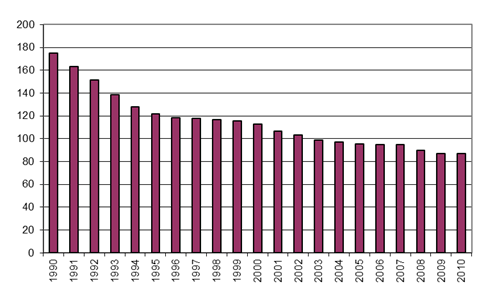
Fig. 5‑1 Trend of NMVOC emissions from Solvent and Other Product Use [Gg NMVOC]

5.1 Source category description

This category includes particularly emissions of NMVOC (ozone precursor) from the use of solvents, which are simultaneously considered to be a source of CO₂ emissions (these solvents are mostly obtained from fossil fuels), as their gradual oxidation in the atmosphere is also a factor. However, the use of solvents is not an important source of CO₂ emissions - in 2009, CO₂ emissions were calculated at the level of 0.274 Mt CO₂.

This category (Solvent and Other Product Use) also includes N₂O emissions from the use of this substance in the food industry (aerosol cans) and in health care (anaesthesia). These not very significant emissions corresponding to 0.75 Gg N₂O were derived from production in the Czech Republic (0.6 Gg N₂O) and from import of N₂O (0.15 Gg N₂O), see (Markvart and Bernauer, 2010, 2011)

So far, in the Czech Republic, no relevant data have been available to distinguish between N₂O used in anaesthesia and for aerosol cans. Therefore, the existing split (50 % for anaesthesia) was based only on a rough estimate.

Now the authors of the study (Markvart and Bernauer, 2011) have managed to perform studies leading to the qualified estimate that approx. 80% of the N₂O is used in medicine (anaesthesia). This estimate applies to the entire 1990 – 2010 time period.

5.2 Methodological aspects

The IPCC methodology (Revised 1996 IPCC Guidelines, 1997) uses the CORINAIR methodology (EMEP / CORINAIR Guidelines, 1999) for processing NMVOC emissions in this category. This manual also gives the following conversions for the relevant activities, which can be used in conversion of data from the CORINAIR (i.e. SNAP) structure to the IPCC classification.

Tab. 5‑1 Conversion from SNAP into IPCC nomenclature

SNAP	SOLVENT AND OTHER PRODUCT USE	IPCC
06 01	Paint application	3A	Paint application
	Items 06.01.01 to 06.01.09
06 02	Degreasing, dry cleaning and electronic	3B	Degreasing and dry cleaning
	Items 06.02.01 to 06.02.04
06 03	Chemical products manufacturing or processing.	3C	Chemical products
	Items 06.03.01 to 06.03.14
06 04	Other use of solvents + related activities	3D	Other
	Items 06.04.01 to 06.04.12
06 05	Use of N₂O	3D	Other
	Items 06.06.01 to 06.06.02

Inventory of NMVOC emissions for 2010 for this sector is based on a study prepared by SVÚOM Ltd. Prague (Geimplová, 2011). This study is elaborated annually for the UNECE / CLRTAP inventory in NFR and is also adopted for the National GHG inventory.

Solvent Use chapter is based on the following sources of information:

· statistical information on producers and imports from the Czech Statistical Office,

· REZZO data,

· annual reports of the Association of Coatings Producers and Association of Industrial Distilleries,

· information from the Customs Administration.

· regular monitoring of economic activities and economic developments in the CR, knowledge and monitoring of important operations in the sphere of surface treatments, especially in the area of application of coatings, degreasing and cleaning;

· regular monitoring of investment activities is performed in the CR for technical branches affecting the consumption of solvents and for overall developmental technical trends of all branches of industry;

· monitoring of implementation of BAT in the individual technical branches;

· technical analysis of consumption of solvents in households; NMVOC emissions from households are entirely fugitive and, according to qualified estimates, contribute approximately 16.5 % to total NMVOC emissions.

The activity data used in the individual categories and subcategories vary considerably. Basic processing of data is performed in a more detailed classification than that used in the CRF Reporter. A survey of the individual groups of products and the formats of the activity data for basic processing of emission data are apparent from the following survey.

It is apparent from the Tab. 5‑2 that uniform expression of the activity data cannot be employed, as this corresponds in the individual cases to consumption of coatings, degreasing agents, solvents and, in some cases, the weight of the final production, e.g. Dry Cleaning. Consequently, total NMVOC emissions are employed as activity data in the CRF Reporter.

NMVOC emissions oxidize relatively rapidly in the atmosphere, so that CO₂ emissions generated as a consequence of this atmospheric oxidation are also reported in CRF. The CO₂ emissions are calculated using a conversion factor that contains the ratio C/NMVOC = 0.855 and a recalculation ratio of C to CO₂ equal to 44/12. The overall conversion factor has a value of 3.14.

Tab. 5‑2 Structure for basic processing of emission data and the dimensions of activity data

A Paint Application	EF - units
PAINT APPLICATION - MANUFACTURE OF AUTOMOBILES	10³ m²
PAINT APPLICATION - CAR REPAIRING	t of paint
PAINT APPLICATION - CONSTRUCTION AND BUILDINGS	t of paint
PAINT APPLICATION - DOMESTIC USE	t of paint
PAINT APPLICATION - COIL COATING	10³ m²
PAINT APPLICATION - WOOD	t of paint
OTHER INDUSTRIAL PAINT APPLICATION	t of paint
OTHER NON INDUSTRIAL PAINT APPLICATION	t of paint
B Degreasing and Dry Cleaning
METAL DEGREASING	t
DRY CLEANING	t
ELECTRONIC COMPONENTS MANUFACTURING	t
OTHER INDUSTRIAL CLEANING	t
C Chemical Products Manufacture / Processing
POLYESTER PROCESSING	t
POLYVINYLCHLORIDE PROCESSING	t
POLYSTYRENE FOAM PROCESSING	t
RUBBER PROCESSING	t
PHARMACEUTICAL PRODUCTS MANUFACTURING	t
PAINTS MANUFACTURING	t
INKS MANUFACTURING	t
GLUES MANUFACTURING	t
ADHESIVE MANUFACTURING	t
ASPHALT BLOWING	t
TEXTILE FINISHING	10³ m²
LEATHER TANNING	10³ m²
D Other	-

5.3 Uncertainty and time consistency

The uncertainty estimates have not yet been reported. Their implementation is ongoing and is planned for inclusion in the following NIR.

Time series consistency is ensured as the inventory approaches concerned are employed identically across the whole reporting period from the base year 1990 to 2010.

5.4 QA/QC and verification

The emission data in this section were taken from the UNECE / CLRTAP inventories in NFR. Annual reports are available on the method of calculation for the individual years from 1998. Following transfer of the emission data to the new CRF Reporter, it was apparent that trends in the emissions for all of Sector 3 – Solvent and Other Product Use – did not exhibit any significant deviations.

A control was performed of the company processing the data (SVÚOM Ltd. Prague) and the coordinator of processing of UNECE / CLRTAP inventories in NFR. It was found that more exact data were available to 2000, permitting assignment of consumption of the individual types of solvents and other preparations containing NMVOC to individual subcategories, from which the emissions are calculated in 4 main subcategories of Sector 3 Solvent and Other Product Use. As the total consumption of substances containing NMVOC in all of CR is relatively well known, from 2000 the emissions that could not be identified in the individual subcategory 3B Decreasing and Dry Cleaning were transferred to Category 3D Other Solvent Use, because they were missing in the overall balance.

5.5 Recalculations

This recalculation can be seen as the reallocation of N₂O emissions for category 3D mentioned at the beginning of this chapter.

5.6 Source-specific planned improvements

The value of the conversion factor (3.14) is slightly higher compared to other countries. It is planned to try to obtain background information for a country-specific value. Because of funding shortage it was not possible to obtain data about carbon content in solvents used in CR.

6 Agriculture (CRF Sector 4)

6.1 Overview of sector

Agricultural greenhouse gas emissions under Czech national conditions consist mainly of emissions from enteric fermentation (CH₄ emissions only), manure management (CH₄ and N₂O emissions) and agricultural soils (N₂O emissions only). The other IPCC subcategories – rice cultivation, prescribed burning of savannas, field burning of agricultural residues and “other” – do not occur in the Czech Republic.

Methane emissions are derived from animal breeding. These are derived primarily from enteric fermentation (digestive processes), which is manifested most for ungulate animals (in this country mostly cattle). Other emissions are derived from fertilizer management, where methane is formed under anaerobic conditions (with simultaneous formation of ammonia which, however, is not monitored in the framework of greenhouse gas inventories).

Nitrous oxide emissions are formed mainly by nitrification-denitrification processes in soils. The anthropogenic contribution that is determined in the national inventory of greenhouse gases is caused by nitrogenous substances derived from inorganic nitrogen-containing fertilizers, manure from animal breeding and nitrogen contained in parts of agricultural crops that are returned to the soil (for example, in the form of straw together with manure, or that are ploughed into the soil). In addition, emissions are also included from stables and fertilizer management and indirect emissions derived from atmospheric deposition and from nitrogenous substances flushed into water courses and reservoirs.

6.1.1 Key categories

For Agriculture, five of six relevant categories of sources were evaluated by analysis decribed in IPCC (2000 and 2003) as the key categories. An overview of sources, including their contribution to aggregate emissions, is given in Tab. 6‑1.

Tab. 6‑1 Overview of significant categories in this sector (2010)

Category		Character of category	Gas	% of total GHG*
4D1	Agricultural soils, direct emissions	KC (LA, TA, LA, TA)	N₂O	2.0
4A	Enteric fermentation	KC (LA, TA, LA, TA)	CH₄	1.4
4D3	Agricultural soils, indirect emissions	KC (LA, TA, LA, TA)	N₂O	1.3
4B	Manure management	KC (LA, TA, LA, TA)	N₂O	0.5
4B	Manure management	KC (TA, TA*)	CH₄	0.3
4D2	Pasture, range and paddock manure	Non-KC	N₂O	0.2

* assessed without considering LULUCF

KC: key category, LA, LA*: identified by level assessment with and without considering LULUCF, respectively

TA, TA*: identified by trend assessment with and without considering LULUCF, respectively

6.1.2 Quantitative overview

Agriculture is the third largest sector in the Czech Republic with 5.8 % of total GHG emissions (incl. LULUCF) in 2010 with 7 777 Gg CO₂eq.; 60.4 % of emissions is coming from Agricultural Soils, 25.7 % from Enteric Fermentation and 13.9 % from Manure Management.

The CH₄ emissions from agriculture present 23 % of total national CH₄ emissions and the N₂O emissions from agriculture present 72 % of total national N₂O emissions in 2010. During period 1990-2010 emissions from Agriculture decreased by almost 50 %. The quantitative overview and emission trends in reported period are provided in Fig.6.1 and Tab. 6.2.

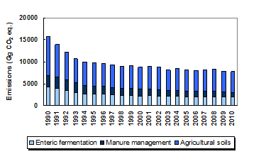
Fig. 6.1 The emission trend in agricultural sector during reporting period 1990–2010 (in Gg CO₂ eq.)

Tab. 6‑2 Emissions of Agriculture in period 1990-2010 (sorted by categories)

Year	Total Emissions	Enteric Fermentation *(4A)*	Manure Management *(4B)*	Agricultural Soils *(4D)*
Year	[Gg CO₂ eq.]
1990	15 733	4 219	2 710	8 804
1991	13 956	3 980	2 585	7 391
1992	12 191	3 568	2 344	6 279
1993	10 686	3 088	2 106	5 491
1994	9 898	2 705	1 862	5 331
1995	9 875	2 632	1 742	5 501
1996	9 540	2 608	1 802	5 130
1997	9 377	2 436	1 745	5 197
1998	8 976	2 284	1 654	5 038
1999	9 053	2 334	1 659	5 060
2000	8 786	2 241	1 544	5 001
2001	8 919	2 257	1 483	5 179
2002	8 706	2 209	1 414	5 083
2003	8 127	2 186	1 351	4 590
2004	8 502	2 139	1 299	5 065
2005	8 135	2 094	1 236	4 804
2006	8 013	2 064	1 218	4 731
2007	8 179	2 084	1 212	4 883
2008	8 374	2 103	1 179	5 091
2009	7 926	2 047	1 107	4 772
2010	7 777	1 999	1 079	4 699

The trend series are consistent both for methane and for nitrous oxide. For methane, the decrease in emissions for enteric fermentation since 1990 is connected with the decrease in the numbers of animals (especially cattle) while the decrease in emissions derived from manure (especially swine manure) is not as great, as there has been a smaller decrease in the number of head of swine. It would seem that conditions have partly stabilized somewhat in agriculture since 1994.

During the in-country review in August/September 2011, the expert review team (ERT) identified the estimation of N₂O emissions from Manure management of dairy cattle as a potential problem. The revision of background information and Nex values for dairy cattle was requested. Already during the review, the Czech Republic introduced revised country-specific data for emission estimation using Tier 2 methods for Manure management of dairy cattle. This recalculation was submitted to ERT as an resolved issue of the “Saturday paper” regarding the 2011 NIR submission.

The assessment review report (UNFCCC/ARR/2011/CZE) provided additional recommendations to improve the inventory estimates for Agriculture. Other country-specific data for non-dairy cattle was obtained. Based on these recommendations and additional country-specific data, the following improvements were implemented in this 2012 submission:

Reallocation of the "Suckler cows" sub-category from Dairy cattle to Non-dairy cattle
More accurate animal population data (not rounded off to thousands) reported (cattle, swine, sheep and poultry).
More accurate data for individual cattle sub-categories (suckler and dairy cows, young heifers, young bulls and calves) reported (not rounded off to thousands) for the period since 2006 (since when the detailed data are available).
Recalculation of N₂O emissions from Manure management using revised and complemented country-specific data: Nex values for cattle, manure type distribution (AWMS), protein in milk and protein in feed. Tier 2 methods implemented for the emission estimation of Manure management of dairy and non-dairy cattle.
Additionally, a new country-specific parameter on digestibility (DE, in %) was determined and implemented in the 2012 submission.

Given that the value of Nex for cattle was revised based on the recommendation of ERT (2011), it led to changes in N₂O emissions from Animal manure applied to soils, Pasture, range and paddocks (PRP), Atmospheric deposition and N-lost through leaching and run-off. These changes apply to the entire reporting period.

The recalculation requested based on the document “Potential problems from ERT (Saturday paper)” led to increased emissions by about 14 % relative to the older approach (submission 2011). The use of updated country-specific data for cattle in calculation of emissions in the 2012 submission resulted in a decrease in emissions by about 1.2 % in 1990 and increase by about 0.6 % in 2009 compared to the 2011 submission.

The following table presents the differences between the emissions in the 2011 and 2012 submissions. Arrows indicate a decrease (↓), or increase (↑) in the values in the 2012 submission compared to the previous 2011 submission (April 2011) in the individual categories between 1990 and 2009.

Tab. 6‑3 Comparison of changes according to previous year

	Total emissions	Enteric Fermentation	Manure Management	Agricultural Soils
1990	1.2 % ↓	13 % ↓	58 % ↑	5.9 % ↓
2009	0.6 % ↑	13 % ↓	49 % ↑	0.1 % ↓
	Manure Management (CH₄)	Manure Management (N₂O)
1990	0.8 % ↓	144 % ↑
2009	6.2 % ↓	126 % ↑
	Manure applied to soils	PRP	Atmospheric deposition	Leaching
1990	11 % ↑	66 % ↓	4 % ↓	3 % ↓
2009	17 % ↑	43 % ↓	2 % ↑	2 % ↑

Note: The significance of the changes depends on the amount of emission values in the individual categories.

6.2 Enteric fermentation (4A)

6.2.1 Source category description

This chapter describes estimation of the CH₄ emissions from Enteric Fermentation. In 2010, 84.4 % of agricultural CH₄emissions arose from this source category (Table 6.2). This category includes emissions from cattle (dairy and non-dairy), swine, sheep, horses and goats. Buffalo, camels and llamas, and mules and asses do not occur in the Czech Republic. Enteric fermentation emissions from poultry have not been estimated, the IPCC Guidelines do not provide a default emission factor for this animal category.

6.2.2 Methodological issues

Emissions from enteric fermentation of domestic livestock have been calculated by using IPCC Tier 1 and Tier 2 methodologies presented in the Revised IPCC Guidelines (IPCC, 1997) and IPCC Good Practice Guidance (IPCC, 2000). Methane emissions for cattle, which are a dominant source in this category, have been calculated using the Tier 2 method, while for other livestock the Tier 1 method was used. The contribution of emissions from livestock other than cattle to the total emissions from enteric fermentation is not significant.

6.2.2.1 Enteric fermentation of cattle

As the most important output of the national study (Kolar, Havlikova and Fott, 2004), a system of calculation spreadsheets have been developed and used for all the relevant calculations of CH₄ emissions.

The emission factor for methane from fermentation (EF) in kg/head p.a. according to the Revised Guidelines (IPCC, 1997) and Good Practice Guidance (IPCC, 2000) is proportional to the daily food intake and the conversion factor. It thus holds that

EF_i = 365 / 55.65 * daily food intake _i * Y

where the “daily food intake” (MJ/day) is taken as the mean feed ration for the given type of cattle (there are several subcategories of cattle) and Y is the conversion facto, which is considered to be Y = 0.06 for cattle. Coefficient 55.65 has dimensions of MJ/kg CH₄.

In principle, this equation should be solved for each cattle subcategory, denoted by index i. The Czech Statistical Office, see Statistical Yearbooks (CzSO, 1990–2010), provides following categorization of cattle:

· Calves younger than 6 months[14] of age (male and female)

· Young bulls and heifers (6-12 months of age[15])

· Bulls and bullocks (1 – 2 years, over 2 years)

· Heifers (1 – 2 years, over 2 years)

· Mature cows (dairy and suckler)

More disaggregated sub-categories given above in parenthesis are given in the study by external agricultural consultants of CHMI (Hons and Mudrik, 2003).

In the calculation, it is also very important to distinguish between dairy and suckler cows, where the fraction of suckler cows (suckler/all cows) gradually increased in the 1990-2010 time period. Based on the ERT recommendation (2011) the sub-category "Suckler cows" was reallocated from Dairy cattle to Non-dairy cattle.

According to the IPCC methodology, Tier 2 (IPCC, 1997 and IPCC, 2000), the “daily food intake” for each subcategory of cattle is not measured directly, but is calculated from national zoo-technical inputs, mainly weight (including the final weight of mature animals), weight gain (for growing animals), daily milk production including the percentage of fat (for cows) and the feeding situation (stall, pasture). The national zoo-technical inputs (noted above) were updated by expert from the Czech University of Agriculture in Prague in 2006 and 2011. Examples of input data used (Hons and Mudřík, 2003, Mudřík and Havránek, 2006, Kvapilík J. 2011) are given below, Tab. 6‑4 and Tab. 6‑5.

Tab. 6‑4 Weights of individual categories of cattle, 1990–2010, in kg

Categories of cattle	1990 – 94	1995 – 98	1999 – 04	2005 – 09	2010 -
Mature cows (dairy and suckler)	520	540	580	585	590
Heifers > 2 years	485	490	505	510	515
Bulls and bullocks > 2 years	750	780	820	840	850
Heifers 1-2 years	380	385	395	395	390
Bulls 1-2 years	490	510	530	540	560
Heifers 6-12 months	275	280	285	285	290*
Bulls 6-12 months	325	330	335	340	540*
Calves to 6 months	128	132	133	135	135*

Note: * Since 2009 the age limit for “Calves” shifted up to 8 months.

Tab. 6‑5 Feeding situation, 1990–2010, in % of pasture, otherwise stall is considered

Categories of cattle	1990 – 94	1995 – 98	1999 – 04	2005 – 09	2010 -
Dairy cows	10	20	20	22	15
Suckler cows	10	20	20	22	95
Heifers > 2 years	30	30	30	35	50
Bulls > 2 years.	30	40	40	40	25
Heifers 1-2 years	30	40	40	40	50
Bulls 1-2 years	30	40	40	40	25
Heifers 6-12 months	30	40	40	40	50*
Bulls 6-12 months	30	40	40	40	50*

Note: * Since 2009 the age limit for “Calves” shifted up to 8 months.

Percentages of pasture are related only to the summer part of the year (180 days), while only the stall type is used in the rest of year. The daily milk production statistics (Tab. 6.5), in which only milk from dairy cows is considered, increased to 18.91 liters/day/head in 2010, with an average fat content of 3.86 %. Milk from suckler cows is not included in the table 6.5; a relevant daily milk production of 3.5 l /day head was used for the calculation. The activity data of milk production comes from the official statistics (CzSO) and these are verified in Yearbook of cattle in Czech Republic (annual report).

As the official statistics, specifically from CzSO, provide population values for cows and other cattle, the resulting EFs in the CRF Tables are defined for the categories of “Dairy cows” and “Non-dairy cattle”, as well as the relevant cells in the CRF. The numbers of animal population are based on surveys of livestock (up to 1991 as at 1.1., from 1992 to 2002 as at 1.3., since 2003 as at 1.4.).

The new country-specific parameter DE (digestibility, in %) for cattle was estimated based on existing publications. Based on the individual OMD (organic matter digestibility) values for the most common feed (e.g. corn silage, hay and straw, green fodder – alfalfa and clover, etc.) the average digestibility for cattle was estimated. The estimated average digestibility corresponds to approximately 70 % (Koukolová and Homolka 2008 and 2010, Tománková and Homolka 2010, Jančík et al. 2010, Petrikovič et al. 2000, Petrikovič and Sommer 2002, Sommer 1994, Zeman 1995 and Zeman et. al. 2006, Třináctý 2009, Čermák et al. 2008). Dr. Pozdíšek (expert from the Research Institute for Cattle Breeding, Ltd., pers. communication) determined the conservative average digestibility values for 3 basic cattle sub-categories. These digestibility values were employed for the emission estimation:

· Dairy cattle DE = 67 %

· Suckler cows DE = 62 %

· Other cattle DE = 65 %

Details of the calculation are given in the above-mentioned study (Kolar, Havlikova and Fott, 2004) and the results are illustrated in Tab. 6‑7. It is obvious that EFs have increased slightly since 1990 because of the increasing weight and milk production for cows and because of the increasing weight and weight gain for other cattle. On the other hand, CH₄ emission from enteric fermentation of cattle dropped during the 1990-2010 period to about one half of the former values due to the rapid decreases in the numbers of animals kept.

Tab. 6‑6 Milk production of dairy cows and fat content (1990–2010)

	Dairy cows	Daily production	Fat content
	[thousands]	[liters / day head]	[%]
1990	1206	10.67	4.03
1991	1165	9.63	4.09
1992	1006	10.13	4.07
1993	902	10.18	4.10
1994	796	10.79	4.04
1995	732	11.34	4.02
1996	713	11.69	4.08
1997	656	11.29	4.02
1998	598	12.44	4.05
1999	583	12.85	4.03
2000	548	13.55	4.00
2001	529	14.00	4.03
2002	496	15.08	3.98
2003	490	15.77	3.98
2004	476	16.41	3.98
2005	438	17.13	3.90
2006	424	17.45	3.90
2007	410	17.94	3.88
2008	406	18.51	3.86
2009	400	18.82	3.85
2010	384	18.91	3.86

6.2.3 Enteric fermentation of other livestock

Compared to cattle, the contribution of other farm animals to the whole CH₄ emissions from enteric fermentation is much smaller, only about 5,5 %. Therefore, CH₄ emissions from enteric fermentation of other farm animals (other than cattle) are estimated by the Tier 1 approach. Because of some features of keeping livestock in the Czech Republic that are similar to the neighbouring countries of Germany and Austria, default EFs for Tier 1 approaches recommended for Western Europe were employed. The obsolete national approach used in the past, which was found not to be comparable with other European countries (Dolejš, 1994 and Jelínek et.al., 1996), was definitively abandoned. The estimated values are presented for the whole period since 1990.

Sheep, goats, swine and horses

The Czech Statistical Office (CzSO) publishes data on the number of goats, sheep, swine, horses and poultry annually in the Statistical Yearbooks (1990-2010).

Considering the rather small numbers in these animal categories, default coefficients from the IPCC method have been used for estimating methane emissions: 8 kg of methane annually per head for sheep, 5 kg of methane for goats, 1.5 kg of methane for swine and 18 kg of methane for horses.

Poultry

IPCC guidelines do not define or require estimates of quantities of methane from enteric fermentation.

Tab. 6‑7 Methane emissions from enteric fermentation, cattle (Tier 2, 1990–2010)

	Dairy cows	Other cattle	EF. cows	EF. other	Em. cows	Em. other	Emissions
	[thous.]	[thous.]	[kg CH₄ / hd]	[kg CH₄ / hd]	[Gg CH₄]	[Gg CH₄]	[Gg CH₄]
1990	1206	2300	82.35	39.25	99.33	90.28	189.61
1991	1165	2195	79.01	39.41	92.08	86.50	178.58
1992	1006	1943	80.67	40.38	81.17	78.48	159.65
1993	902	1609	80.96	40.08	73.06	64.49	137.56
1994	796	1366	82.81	40.03	65.90	54.67	120.56
1995	732	1298	86.29	41.98	63.18	54.47	117.66
1996	713	1275	87.78	42.28	62.63	53.91	116.55
1997	656	1210	86.09	42.88	56.50	51.87	108.37
1998	598	1103	90.27	43.04	53.97	47.48	101.44
1999	583	1074	94.16	45.57	54.90	48.96	103.86
2000	548	1026	96.42	45.92	52.82	47.10	99.92
2001	529	1053	98.17	46.52	51.97	48.98	100.96
2002	496	1024	101.59	47.29	50.42	48.42	98.83
2003	490	984	103.98	47.60	50.99	46.81	97.80
2004	476	952	106.20	47.53	50.54	45.27	95.80
2005	438	960	108.46	48.31	47.49	46.36	93.84
2006	424	950	109.56	48.35	46.45	45.91	92.36
2007	410	981	111.07	48.45	45.58	47.53	93.11
2008	406	996	112.85	48.88	45.76	48.69	94.45
2009	400	964	113.82	48.77	45.47	47.00	92.47
2010	384	966	114.26	47.91	43.82	46.27	90.09

6.2.4 Uncertainty and time-series consistency

As mentioned above, methane emissions from the breeding of farm animals are caused both by enteric fermentation and also by the decomposition of animal excrements (manure). Determination of these emissions was prepared at the level of both Tier 1 and Tier 2. As enteric fermentation is considered according to Tab. 6.1 to constitute a key source, preference should be given to determination in Tier 2.

For quite a long time, calculations were based on historical studies (Dolejš, 1994) and (Jelínek et al, 1996). In principle, emissions from animal excrements could be calculated according to Tier 1 (this is not a key source); however, because of tradition and for consistency of the time series, the final values were also calculated according to Tier 2 using the emission factors from above-mentioned studies (Dolejš, 1994; Jelínek et al, 1996). An approach based on historical studies was indicated to be obsolete in many reviews organized by UNFCCC. Moreover, IEFs (implied emission factors) were mostly found as outliers: especially EFs for enteric fermentation in cattle seemed to be substantially underestimated. Details of the historical approach are given in former NIRs (submitted before 2006).

The Czech team accepted critical remarks put forth by the International Review Teams (ERT) and prepared a new concept for calculation of CH₄ emissions. This concept, in accordance with the plan for implementing Good Practice, is based on the following options:

1) Emissions of methane from enteric fermentation of livestock (a key source) come predominantly from cattle. Therefore Tier 2, as described in Good Practice (Good Practice Guidance, 2000) is applied only to cattle.

2) CH₄ emissions from enteric fermentations of other farm animals are estimated by the Tier 1 approach. Because of some features of keeping livestock in the Czech Republic that are similar to the neighbouring countries of Germany and Austria, default EFs for Tier 1 approaches recommended for Western Europe were employed.

Increased attention was first paid to enteric fermentation. It was stated that cooperation with specialized agricultural experts is crucial to obtain new consistent and comparable data of suitable quality. The relevant nationally specific data, milk production, weight, weight gain for growing animals, type of stabling, etc. were collected by our external experts (Hons and Mudrik, 2003). Moreover, statistical data for sufficiently detailed classification of cattle, which are available in the Czech Republic, were also collected at the same time. Calculation of enteric fermentation of cattle using the Tier 2 approach was described in a study (Kolar, Havlikova and Fott, 2004) for the whole time series since 1990 using the above-mentioned country-specific data. The necessary QA/QC procedures were performed in cooperation with experts from IFER. The nationally specific data like weight of individual categories of cattle, weight gains of these categories and recent feeding situation were revised in 2006. The new values were estimated in a similar way by our external experts (Mudrik and Havranek, 2006) for the next period.

The national zoo-technical inputs (mainly weight, weight gain, daily milk production including the percentage of fat and the feeding situation) were updated in this submission in conjunction with an expert from the Research Institute of Animal Production.

Also in this submission, the sub-category "Suckler cows" was reallocated from “Dairy cattle” to “Non-dairy cattle”; more accurate cattle population data was used. Additionally, the new digestibility values (DE) were employed for cattle (detailed in Chapter 6.2.2.1), affecting the implied emission factors for cattle categories. These changes in the activity data and input parameters resulted in changes in emissions for the entire reporting period.

Uncertainty estimates based on expert judgement.

The uncertainty in the activity data equals 5 %.

The uncertainty in the emission factor equals 20 %.

The combined uncertainty, calculated according to IPCC GPG Tier 1 methodology, equals 20.6 %.

6.2.5 Source-specific QA/QC and verification

A detailed description of source-specific QA/QC and inventory verification of agriculture is presented in the Chapter 6.5.

6.2.6 Source-specific recalculations

Reallocation of the sub-category Suckler cows from Dairy cattle to Non-dairy cattle was performed in the 2012 submission.

Also more accurate animal population data (not off to thousands) of cattle, swine, sheep, poultry was used for the entire period and more precise data for cattle populations (cattle sub-categories) are reported (not rounded off to thousands) since 2006 where data are available.

Last but not least, the new digestibility values (DE) were employed for cattle (dairy cows, suckler cows and other cattle).

These changes in the activity data and input parameters resulted in changes in emissions for the entire reporting period.

6.2.7 Planned improvements

The analysis of uncertainties is currently in progress.

6.3 Manure management (4B)

This chapter describes the estimation of CH₄ and N₂O emissions from animal manure. In 2010, 16.6 % of agricultural CH₄ emissions (18.91 Gg CH₄) and 12.7 % of agricultural N₂O emissions (2.20 Gg N₂O) were caused by this source category. Total emissions from Manure Management are 1079.23 Gg CO₂eq. in 2010.

6.3.1 Source category description

During period 1990-2010 emissions from Manure Management decreased by 60 %. Emissions from cattle and swine dominate the trend (see Tab. 6.7). The reduction in the cow population is partly counterbalanced by an increase in cow efficiency (increasing gross energy intake and milk production).

This emission source covers manure management of domestic livestock. Both nitrous oxide (N₂O) and methane (CH₄) emissions from manure management of livestock (cattle, swine, sheep, horses, goats and poultry) are reported. The animal waste management systems (AWMS) are distinguished for N₂O emission estimations: liquid system, daily spread, solid storage & dry lot and other manure management systems. Nitrous oxide is produced by the combined nitrification-denitrification processes occurring in the manure nitrogen. Methane is produced in manure during decomposition of organic material by anaerobic and facultative bacteria under anaerobic conditions. The amount of emissions is dependent on the amount of organic material in the manure and climatic conditions.

Tab. 6‑8 Emissions of Manure Management in reporting period 1990-2010.

Year	Emissions from Manure Management
	CH₄ emissions		N₂O emissions
	[Gg CH₄]	[Gg CO₂ eq.]	[Gg N₂O]	[Gg CO₂ eq.]
1990	47.68	1001.19	5.51	1708.42
1991	45.91	964.07	5.23	1621.43
1992	42.07	883.54	4.71	1460.79
1993	38.37	805.72	4.19	1300.32
1994	33.56	704.82	3.73	1157.37
1995	31.78	667.38	3.47	1074.20
1996	31.92	670.34	3.65	1131.20
1997	30.89	648.67	3.54	1096.25
1998	29.34	616.19	3.35	1038.31
1999	29.02	609.42	3.39	1049.53
2000	27.34	574.18	3.13	970.10
2001	26.45	555.36	2.99	927.67
2002	25.80	541.78	2.81	872.14
2003	25.00	524.98	2.67	826.25
2004	23.80	499.73	2.58	799.00
2005	22.55	473.62	2.46	762.87
2006	22.22	466.71	2.42	751.01
2007	22.11	464.27	2.41	748.01
2008	21.16	444.32	2.37	735.10
2009	19.43	408.07	2.26	699.20
2010	18.91	397.13	2.20	682.20

6.3.2 Methodological issues

6.3.2.1 Methane emissions

CH₄ emissions from manure management were identified as a key source only by trend assessment (TA); hence these emissions for all farm animals are estimated by the Tier 1 approach. Default EFs for Western Europe were employed for similar reasons as in the previous paragraph (Tab. 6‑9). Similarly as for enteric fermentation, the obsolete national approach used in the past was abandoned because of lack of comparability with other countries. Relation to the decreasing trend in animal population (especially cattle and swine, Fig. 6.2), the emissions from Manure Management rapidly declined during 1990-2010.

Tab. 6‑9 Table 6.8 IPCC default emission factors used to estimate CH₄ emissions from Manure Management

Livestock type	EF (kg/head/yr)
Dairy Cattle	14
Non-Dairy Cattle	6
Sheep	0.19
Goats	0.12
Horses	1.39
Swine	3
Poultry	0.078

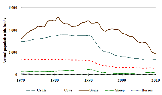
Fig. 6.2 Trend of individual animal population in period 1970–2010

6.3.2.2 Nitrous oxide emissions

N₂O emissions from manure management were identified as a key source; Tier 2 methodology is used for emission estimation for the cattle category (Tier 2 for other animals). Emissions are calculated on the basis of N excretion per animal and animal waste management system. Following the guidelines, all emissions of N₂O taking place before the manure is applied to soils are reported under Manure Management. The IPCC Guidelines method for estimating N₂O emissions from manure management entails multiplying the total amount of N excretion (from all animal species/categories) in each type of manure management system by an emission factor for that type of manure management system.

In response to the list of potential problems and further questions raised by the ERT, the Czech Republic revised the Nex values for dairy and non-dairy cattle (see Tab. 6‑10) and changed the distribution ratio of manure per AWMS (see Tab. 6‑11) according to the national conditions based on expert judgment (Hons and Mudřík 2004 and Kvapilík J. 2011).

The IPCC default nitrogen excretion (Nex) values and distribution of AWMS systems for other animal categories (excl. cattle) are presented in Tab. 6‑12. According to GPG (IPCC, 2000), the IPCC default values for swine were taken from Tables B-3 through B-6 and the IPCC default values for all the other animal species were taken from Table 4-21. The emissions are then summed over all the manure management systems.

Tab. 6‑10 Czech national Nex (nitrogen excretion) values used to estimate N₂O emissions from Manure Management

Year	Nitrogen excretion (Nex)
	Dairy cows	Non-dairy cattle (AVG value)
	[kg/head/year]
1990	101.94	58.51
1991	99.06	58.66
1992	100.51	59.66
1993	100.85	59.17
1994	102.38	59.09
1995	105.93	61.27
1996	107.45	61.61
1997	105.75	62.28
1998	109.63	62.52
1999	114.61	65.43
2000	116.57	65.87
2001	118.26	66.58
2002	121.16	67.47
2003	123.33	67.90
2004	125.32	67.78
2005	127.15	69.00
2006	128.13	69.00
2007	129.39	69.00
2008	130.89	69.51
2009	131.71	69.49
2010	132.59	68.76

Tab. 6‑11 Czech national distribution of AWMS systems for cattle categories only

Dairy cows	Fraction of Manure Nitrogen per AWMS (in %)
Dairy cows	Liquid	Daily spread	Solid	PRP
1990	25	2	68	5
1995	23	1	66	10
2000	15	1	74	10
2005	26	1	62	11
2010	27	1	65	7
Non-dairy cattle (AVG)	Liquid	Daily spread	Solid	PRP
1990	51	1	33	15
1995	48	1	31	20
2000	49	1	33	17
2005	52	1	27	20
2010	52	1	27	20

Tab. 6‑12 IPCC default nitrogen excretion (Nex) and distribution of AWMS systems for other animal categories (excl. cattle)

Livestock type	Nex (kg/head/yr)	Type of AWMS
		Liquid	Daily spread	Solid	PRP	Other
		Fraction of Manure Nitrogen per AWMS (in %)
Sheep	20	0	0	2	87	11
Swine	20	76	0	23	0	1
Poultry	0.6	13	0	1	2	84
Horses	25	0	0	0	96	4
Goats	25	0	0	0	96	4

6.3.2.3 Emission factors

To estimate N₂O emissions from manure management, the default emission factors for the different animal waste management systems were taken from the Good Practice Guidance, Table 4-22 (IPCC, 2000), see Tab. 6‑13.

Tab. 6‑13 IPCC default emission factors of animal waste per different AWMS

AWMS	Emission Factor (EF3) (kg N₂O-N per kg N excreted)
Liquid	0.001
Solid Storage	0.02
Pasture/Range/Paddock	0.02
Other Systems	0.005

6.3.3 Uncertainty and t ime-series consistency

As mentioned above, methane emissions from the breeding of farm animals are caused both by enteric fermentation and also by the decomposition of animal excrements (manure). Determination of the second of them was prepared at the level Tier 1, besides the cattle where the emissions are calculated by Tier 2 since submission 2012.

The Czech team accepted critical remarks put forth by the International Review Teams (ERT). A concept, in accordance with the plan for implementing Good Practice, is based on option, that CH₄ emissions from manure management for all farm animals are estimated by the Tier 1 approach. For similar reasons as in the previous paragraphs, the default emission factors for Western Europe were employed.

On the basis of the recommendations of the ERT 2009, the estimation of manure management N₂O emissions from horses and goats is reported as two individual groups of animals (category Other livestock was regrouped to two categories), applying the IPCC Tier 1 method and the 1996 IPCC default values. The total emissions from the category “N₂O emissions from Manure Management” were not affected.

According to the recommendations of ERT 2011 (ARR), the recalculation of emissions from Manure Management was performed using new national parameters: feed consumption, nitrogen feed intake and protein content of milk and feed (revised Nex value). In addition, the values of digestible energy expressed as a percentage of gross energy (DE) for cattle were revised (the default values were substituted by national values). In addition, national data on the distribution of manure management practices across AWMS were collected and updated (Kvapilík J. 2011).

Uncertainty estimates based on expert judgement.

The uncertainty in the activity data equals 5 %.

The uncertainty in the emission factor for estimation of CH₄ emissions equals 30 %; for estimation of N₂O emissions, this value equals 100 %.

The combined uncertainty for CH₄ emissions equals 30.4 % and that for N₂O emissions equals 100.12 %.

6.3.4 Source-specific QA/QC and verification

A detailed description of source-specific QA/QC and inventory verification of agriculture is presented in the Chapter 6.5.

6.3.5 Source-specific recalculations

Based on new zoo-technical data and updated country-specific parameters and activity data the emissions from Manure management of for dairy and non-dairy cattle categories were calculated by Tier 2 method over the entire 1990-2010 reporting period.

The estimation of N₂O emissions from Manure management was performed using the revised Nex values for dairy and non-dairy cattle with the updated parameters (feed consumption, nitrogen feed intake and protein content of milk, to estimate the amount of N retained in milk). Equations 10.32 and 10.33 (2006 IPCC) were used to revise Nex and to calculate the variables for nitrogen intake and nitrogen retained (milk production and growth). The results served as an input for Eq. 10.31.

The parameters for estimation of the revised Nex for cattle were collected from literature and from personal communications with agricultural experts. The protein content in milk was determined based on 3.3 % (Poustka 2007, Ingr 2003 and Turek 2000) and protein content in feed (in dry matter) of 18 % (Zeman - Czech feed standards 12-21 %, Central Institute for Supervising and Testing in Agriculture 18 %, Karabcová pers. commun. 16-18 %).

Country-specific redistribution of manure management practices across AWMS for cattle (Tab. 6‑11) was taken from Hons and Mudrik (2004) for the 1990-1999 period and updated data from Kvapilík J. (2011) was used for the 2000-2010 period. Dr. Kvapilik (author of the Annual report of Czech cattle breeding of the Institute of Animal Science in Prague) also provided national data on grazing animals (feed situation of cattle categories, see Tab. 6‑5).

Using the above changes, the N₂O emissions from Manure management were calculated by the Tier 2 method for dairy and non-dairy cattle categories for the entire reporting period.

6.3.6 Planned improvements

The analysis of uncertainties is in progress.

In the next submission the attention will be paid to the using a higher –tier method to estimate CH₄ emissions from Manure Management as recommended by ERT.

6.4 Agricultural Soils (4D)

6.4.1 Source category description

This source category includes direct and indirect nitrous oxide emissions from agricultural soils. Both these categories (direct and indirect) of N₂O soil emissions are the key sources (Tab. 6‑1). Nitrous oxide is produced in agricultural soil as a result of microbial nitrification-denitrification processes. The processes are influenced by chemical and physical characteristics (availability of mineral N substrates and carbon, soil moisture, temperature and pH). Thus, addition of mineral nitrogen in the form of synthetic fertilizers, animal manure applied to soils, crop residue, N-fixing crops enhance the formation of nitrous oxide emissions.

Nitrous oxide emissions from agriculture include these subcategories:

direct emissions (emissions from synthetic fertilizers, animal manure applied to soils, crop residue and N-fixing crops)
emissions from pasture manure (PRP)
indirect emissions (emissions from atmospheric deposition and nitrogenous substances flushed into water courses and reservoirs - leaching)

Tab. 6‑14 N₂O emissions come from Agricultural Soils (4D category) in period 1990-2010 in Gg N₂O.

Year	Total emissions	Direct emissions				Pasture Manure	Indirect emissions
Year	Total emissions	a	b	c	d	Pasture Manure	Atmosph. deposition	Leaching
1990	28.40	7.39	5.50	0.18	3.00	1.02	1.86	9.44
1991	23.84	5.26	5.25	0.24	2.67	0.99	1.62	7.82
1992	20.26	4.00	4.85	0.24	2.26	0.87	1.41	6.63
1993	17.71	3.19	4.38	0.27	2.24	0.72	1.23	5.68
1994	17.20	3.59	3.84	0.19	2.30	0.61	1.15	5.51
1995	17.75	4.05	3.61	0.17	2.23	0.80	1.16	5.71
1996	16.55	3.36	3.64	0.16	2.24	0.78	1.10	5.26
1997	16.76	3.64	3.51	0.12	2.33	0.73	1.10	5.33
1998	16.25	3.59	3.37	0.16	2.25	0.67	1.06	5.17
1999	16.32	3.54	3.41	0.14	2.32	0.67	1.06	5.17
2000	16.13	3.77	3.24	0.10	2.15	0.65	1.05	5.18
2001	16.71	3.99	3.17	0.11	2.44	0.65	1.05	5.28
2002	16.40	4.02	3.12	0.08	2.24	0.63	1.04	5.26
2003	14.81	3.39	3.05	0.09	1.92	0.62	0.97	4.78
2004	16.34	3.83	2.92	0.12	2.91	0.61	0.98	4.97
2005	15.50	3.65	2.80	0.14	2.56	0.64	0.95	4.77
2006	15.26	3.80	2.76	0.12	2.14	0.63	0.95	4.85
2007	15.75	3.95	2.76	0.09	2.37	0.65	0.97	4.95
2008	16.42	4.21	2.68	0.07	2.75	0.67	0.98	5.07
2009	15.39	3.92	2.49	0.09	2.59	0.66	0.91	4.73
2010	15.16	4.00	2.36	0.09	2.28	0.80	0.91	4.73

Note: a, b, c, d = individual sources of direct emissions; (a) Synthetic fertilizers, (b) Animal manure applied to soils, (c) N-fixing crops and (d) Crop residue

In 2010, 87.3 % of total N₂O emissions from Agriculture originated from Agricultural Soils, while the rest originated from Manure Management (12.7 %). The trend in N₂O emissions from this category is decreasing: in 2010 emissions (4699.23 Gg CO₂ eq.) were ca. 47 % below the base year level. Tab. 6‑14 and Figure 6.3 present the N₂O emissions of Agricultural soils by individual sub-category.

Fig. 6.3 Nitrous oxide emissions from Agricultural soils (sub-categories)

6.4.2 Methodological issues

Although nitrous oxide emissions from agriculture are key sources, emissions are estimated and analyzed by the Tier 1 approach of the IPCC methodology (IPCC, 1997). A set of interconnected spreadsheets in MS Excel has been used for the relevant calculations for several years. The emissions from nitrogen excreted to pasture range and paddocks by animals are reported under animal production in CRF table 4D2. The nitrogen from manure that is spread daily is consistently included in the manure nitrogen applied to soils.

6.4.2.1 Activity data

The standard calculation of Tier 1 required the following input information based on CzSO data:

· number of heads of farm animals (dairy cows, other cattle, pigs, sheep, poultry, horses and goats),

· annual amount of nitrogen applied in the form of industrial nitrogen fertilizers - the application of agricultural fertilizers was previously intensive in this country, but decreased radically during the 1990s. The amount of nitrogen fertilizers applied in 1990 equaled over 418 kt decreased to 226 kt in 2010. This corresponds to the trend reported for use of fertilizers, which decreased a lot in early 1990s (Sálusová et al., 2006).

· annual harvests of crops, pulses and soya beans (see Tab. 6‑15).

All these data were taken from the Statistical Yearbooks of the Czech Republic (Statistical Yearbooks, 1990-2010).

Other input data consists in the mass fraction X_i,j of animal excrement in animal category i (i = dairy cows, other cattle, pigs, …) for various types of excrement management (AWMS - Animal Waste Management System) j (j = anaerobic lagoons, liquid manure, solid manure, pasturage, daily spreading in fields, other). Here, it holds that X_i,1 + X_i,2 + ... + X_i,6 = 1. For Tier 1, (Revised 1996 IPCC Guidelines, 1997) gives only the values of matrix X for typical means of management of animal excrement in Eastern and Western Europe. As we are aware that agricultural farming in the Czech Republic has not yet been classified according to this system, we performed the calculation for AWMS parameters presented in the IPCC methodology (Revised 1996 IPCC Guidelines, 1997) for the case of Western Europe. Nevertheless, collection of the relevant country specific AWMS parameters is under way and perhaps it will be possible to employ such an approach sometime in the future.

Tab. 6‑15 Annual harvests of agricultural products (incl. crops, pulses and soybeans) in period 1990-2010

Year	Crop production	Pulses (excl. soya)	Soya beans
Year	[in thousands tons]
1990	8 947	152	2.2
1991	7 845	195	6.4
1992	6 565	203	3.7
1993	6 468	227	0.7
1994	6 777	163	0.7
1995	6 602	144	0.6
1996	6 644	136	0.5
1997	6 983	104	0.3
1998	6 669	133	0.3
1999	6 928	119	0.6
2000	6 454	85	2.3
2001	7 338	91	4.3
2002	6 771	65	6.4
2003	5 762	62	11.9
2004	8 784	88	12.9
2005	7 660	96	18.9
2006	6 386	88	17.8
2007	7 153	65	13.2
2008	8 370	48	9.4
2009	7 832	62	13.6
2010	6 878	58	16.1

6.4.2.2 Emission factors and other parameters

IPCC default emission factors have been used for calculating N₂O emissions from agricultural soils. The emission factors for calculation of direct N₂O emissions from the agriculture soil category, direct emissions from atmospheric deposition and leaching were used according to Tab. 6‑16.

The default fraction values were used to estimate emissions (Tab. 6‑17). The fraction of livestock N excreted and deposited onto soil during grazing (Frac_GRAZ) varied from 0.085 in 1990 to 0.145 in 2010.

Tab. 6‑16 IPCC default parameters/fractions used for emission estimation

Parameters/Fractions	Default values
Frac_GASM	0.20
Frac_NCR0	0.015
Frac_NCRBF	0.03
Frac_R	0.45
Frac_BURN	0.00

Tab. 6‑17 Emission factors (EFs) for the calculation of Agricultural Soils

	Emissions (sources)	Emission Factors
Direct emissions	Synthetic fertilizer	EF₁=0.0125 kg N₂O-N/kg N
	Animal Waste
	N-fixing crops
	Crop residue
Pasture, range & paddock manure	Grazing animals	EF₃=0.02 kg N₂O-N/kg N
Indirect emissions	Atmospheric Deposition	EF₄=0.01 kg N₂O-per kg emitted NH₃ and NO_x
Indirect emissions	Nitrogen Leaching	EF₅=0.025 kg N₂O - per kg of leaching N

6.4.3 Uncertainty and time-series consistency

In relation to the consistency of the emission series for N₂O (agricultural soils), it should be mentioned that emission estimates have been calculated in a consistent manner since 1996 according to the default methodology of Revised 1996 IPCC Guidelines (IPCC, 1997). Emission estimates for 1990, 1992, 1994 and 1995 were obtained and reported in several recent years; the data for 1991 and 1993 are reported (together with year 2004) this year as part of the 2006 submission.

The quantitative overview and emission trends during period 1990-2010 are shown in Tab. 6.2. The trend in N₂O emissions from agricultural soils is summarized in Tab. 6.15. During 1990-2010 the total emissions from agricultural soils decreased by 47 % (rapidly during period 1990-1995, about 40 %), direct emissions decreased by 40 % and indirect emissions by 50 %. More than 60 % reduction was reached in the animal production.

Following the ERT, the Czech emission inventory team verified the activity data required for this category and found that the previously reported data based on expert judgment of areas could not be confirmed and verified from the official statistics. According to the expert common consensus (I. Skorepova, P. Fott, E. Cienciala and Z. Exnerova), there are no cultivated histosols on agricultural land in this country and hence also no data for this category. Organic soils mostly occur on forest land and they are reported in the LULUCF sector. During in-country review 2009 was confirmed that there are no cultivated histosols on agricultural land in the Czech Republic.

On the basis of the recommendations of ERT (in-country review 2009) and the ARR (2009), several recalculations were performed (N₂O emissions from Animal manure applied to soils, Crop residues, N-fixing crops) and technical errors were corrected in the emission inventory of agricultural soils in the last 2010 submission.

Given that the value of Nex for cattle was revised based on the recommendation of ERT (2011), it led to changes in N₂O emissions from i) animal manure applied to soils (4D1b), ii) PRP (4D2), iii) atmospheric deposition (4D3.1) and iv) N lost through leaching and run-off (4D3.2). These changes apply to the entire reporting period.

Uncertainty estimates based on expert judgement.

The uncertainty in the activity data for estimation of direct and indirect emissions from agricultural soils equals 20 %; for Pasture, Range and Paddock Manure (PRP) this value equals 10 %.

The uncertainty in the emission factor for estimation of direct and indirect emissions from agricultural soils equals 50 %; for estimation of emissions from PRP Manure this value equals 100 %.

The combined uncertainty for the direct and indirect emissions from agricultural soils equals 53.85 %; for N₂O emissions from PRP Manure this value equals 100.5 %.

6.4.4 Source-specific QA/QC and verification

A detailed description of source-specific QA/QC and inventory verification of agriculture is presented in the Chapter 6.5.

6.4.5 Source-specific recalculations

On the basis of the recommendations of ERT (in-country review in August-Sept 2011 in Prague) and the following ARR document, N₂O emissions from agricultural soils were recalculated in the 2012 submission. Given that the value of Nex for cattle was revised in the Manure Management category, it led to changes in N₂O emissions from:

1. animal manure applied to soils (4D1b)

2. pasture, range and paddocks (4D2)

3. atmospheric deposition (4D3.1)

4. nitrogen lost through leaching and run-off (4D3.2)

These changes apply to the entire reporting period.

6.4.6 Planned improvements

The analysis of uncertainties is in progress.

6.5 Source-specific QA/QC and verification

Following the recommendation of the latest in-country review, a sector-specific QA/QC plan was formulated, tightly linked to the corresponding QA/QC plan of the National Inventory System, chapter 1.5. The plan describes the key procedures of inventory compilation, provides a table of personal responsibilities and a timetable of sector-specific QA/QC procedures. This plan consolidates the quality assurance procedures and facilitates effective quality control of the Agriculture inventory.

The Institute of Forest Ecosystem Research (IFER) is the sector-solving institution for this category.

The agricultural greenhouse gas inventory is compiled by an experienced expert from the IFER, including performance of self-control. Czech University of Life Sciences, Institute of Animal Science Prague, Research Institute for Cattle Breeding and the AGROBIO are other institutes contributing information used in the sector of Agriculture. Slovak agricultural experts (SHMI) also participate in debates on inventory improvements.

Potential errors and inconsistencies are documented and corrections are made if necessary. In addition to the official review process, emission inventory methods and results are internally reviewed by the technical experts involved in the emission inventory of the Agriculture and LULUCF sectors.

To comply with QA/QC, is necessary to check

· The inclusion of all activity data for animal categories, selected harvests (crops, pulses, soya beans), amount of synthetic fertilizers (agricultural statistics)

· The consistency of time-series activity data and emission factors (agricultural statistics)

· The annual update of national zoo-technical data

· All the emission factors and used parameters/fractions

QA/QC includes checking of activity data, emission factors and methods employed. All the differences are discussed and, if necessary, also corrected. The procedure of inventory compiling is initiated by IFER, where all the necessary data, obtained from the Czech Statistical Office (CzSO), are inserted into the excel spreadsheets. The excel files are verified by other IFER experts. Some more specific parameters, not available from CzSO, are required to estimate the country-specific emission factors for cattle (Tier 2). The zoo-technical national data (specifically concerned with cattle breeding) are supplied by experts from agricultural institute (see above). The appropriate values in the calculation spreadsheets are updated at IFER, replacing the older values. The verified data are transferred to the CRF Reporter, where the data are again technically verified. The CRF tables are sent to the NIS coordinator for final time-series checking and approval.

All the information used for the inventory report is archived by the author and by the NIS coordinator. Hence, all the background data and calculations are verifiable.

7 Land Use, Land-Use Change and Forestry (CRF Sector 5)

7.1 Overview

The emission inventory of the 5 Land Use, Land Use Change and Forestry (LULUCF) sector includes emissions and removals of greenhouse gases (GHG) resulting from land use, land-use change and forestry. The inventory is based on application of the IPCC Good Practice Guidance for Land Use, Land-Use Change and Forestry (IPCC 2003, further also abbreviated as GPG for LULUCF) and the reporting format adopted by the 9^th Conference of Parties to UNFCCC. The application of GPG for LULUCF in the national emission inventory entails manifold specific requirements on the inventory of the sector, which have been implemented gradually. The current inventory of the LULUCF sector represents an advanced phase of this implementation. It employs a refined system of land use identification at the level of the individual cadastral units, which was also utilized for determination of land-use changes. This inventory submission contains additional methodological improvements and to some degree reflects the suggestions following from the latest reviews of the LULUCF emission inventory. Where feasible, the methodological elements from IPCC 2006 Guidelines for National Greenhouse Gas Inventories (IPCC 2006) for the Agriculture, Forestry and Other Land Use (AFOLU) were also used. Although the Czech LULUCF inventory is still expected to undergo further development and consolidation, it already represents a solid system for providing information on GHG emissions and removals in the LULUCF sector, as well as for providing the additional information on the LULUCF activities required under the Kyoto protocol.

The current inventory includes CO₂ emissions and removals, and emissions of non-CO₂ gases (CH₄, N₂O, NO_x and CO) from biomass burned in forestry and disturbances associated with land-use conversion. The inventory covers all six major LULUCF land-use categories, namely 5A Forest Land, 5B Cropland, 5C Grassland, 5D Wetlands, 5E Settlements and 5F Other Land, which were linked to the Czech cadastral classification of lands. The emissions and/or removals of greenhouse-gases are reported for all mandatory categories. The current submission covers the whole reporting period from the base year of 1990 to 2010 (Fig. 7‑1).

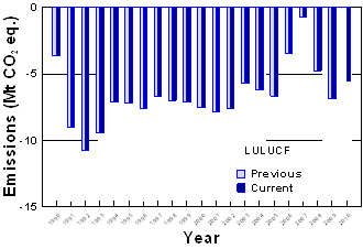
Fig. 7‑1 Current and previously reported assessment of emissions for the LULUCF sector. The values are negative, hence representing net removals of green-house gases.

7.1.1 Estimated emissions

Tab. 7.1 provides a summary of the LULUCF GHG estimates for the base year 1990 and the most recently reported year 2010. In 2010, the net GHG flux for the LULUCF sector, estimated as the sum of emissions and removals, equaled -5.519 Mt CO₂ eq., thus representing a net removal of GHG gases. In relation to the estimated emissions in other sectors in the country for the inventory year 2010, the removals realized within the LULUCF sector decrease the GHG emissions generated in other sectors by 3.97 %. Correspondingly, for the base year of 1990, the total emissions and removals in the LULUCF sector equaled -3.618 Mt CO₂.eq. In relation to the emissions generated in all other sectors, the inclusion of the LULUCF estimate reduces the total emissions by 1.85 % for the base year of 1990. It is important to note that the emissions within the LULUCF sector exhibit high inter-annual variability (Fig. 7.1) and the values shown in Tab. 7.1 should not be interpreted as trends. The entire data series can be found in the corresponding CRF Tables.

Tab. 7.1 GHG estimates in Sector 5 (LULUCF) and its categories in 1990 (base year) and 2010.

Sector/category	Emissions 1990 Gg CO₂ eq.	Emissions 2010 Gg CO₂ eq.
5 Total LULUCF	-3 618	-5 519
5A Forest Land	-4 947	-5 400
5A1 Forest Land remaining Forest Land	-4 667	-5 132
5A2 Land converted to Forest Land	-280	-308
5B Cropland	1 337	139
5B1 Cropland remaining Cropland	1089	38
5B2 Land converted to Cropland	247	101
5C Grassland	-128	-371
5C1 Grassland remaining Grassland	59	2
5C2 Land converted to Grassland	-187	-373
5D Wetlands	23	34
5D1 Wetlands remaining Wetlands	(0)	(0)
5D2 Land converted to Wetlands	23	34
5E Settlements	86	118
5E1 Settlements remaining Settlements	(0)	(0)
5E2 Land converted to Settlements	86	103
5F Other Land	(0)	(0)

Note: Emissions of non-CO₂ gases (CH₄ and N₂O) are also included.

7.1.2 Key categories

Tab. 7.2 Key categories of the LULUCF sector (2010)

Category	Character of category	Gas	% of total GHG
5A1 Forest Land remaining Forest Land	KC (LA, TA)	CO₂	-3.96
5B1 Cropland remaining Cropland	KC (TA)	CO₂	0.03

KC: key category, LA - identified by level assessment, TA - identified by trend assessment

% of total GHG: relative contribution of category to net GHG (including LULUCF)

Of the main categories listed in Tab. 7.1, two of them were identified as key categories according to the IPCC Good Practice (Good Practice Guidance, IPCC 2000, Good Practice Guidance for LULUCF, IPCC 2003). Of these LULUCF categories, the largest effect on the overall emission inventory in the country is attributed to 5A1 Forest Land remaining Forest Land. With a contribution of -4.0 %, it is the only LULUCF category identified by the level assessment for the year 2010 (Tab. 7.2). It was also identified as a key category by the trend assessment. The emissions of this category are determined by the changes in biomass carbon stock. Additionally, one LULUCF category was identified by the trend assessment, namely 5B1 Cropland remaining Cropland (Tab. 7.2). In 5B1, the trend analysis reflected the effect of liming on emissions from agricultural soils, which decreased rapidly in early 1990s compared to the following years.

7.2 General methodological issues

7.2.1 Methodology for representing land-use areas

The reporting format requires the estimation of GHG emissions into the atmosphere by sources and sinks for six land-use categories, namely Forest Land, Cropland, Grassland, Wetlands, Settlements and Other Land. Each of these categories is divided into lands remaining in the given category during the inventory year, and lands that are newly converted into the category from a different one. Accordingly, GPG for LULUCF outlines the appropriate methodologies for estimation of emissions.

Consistent representation of land areas and identification of land-use changes constitute the key steps in the inventory of the sector in accordance with GPG for LULUCF. The adopted land-use representation and land-use change identification system was build gradually since the 2007 NIR submission. It was radically improved in the 2008 NIR submission and further refined in 2009 inventory submission.

Initially, the identification of land-use categories was based on two key data sources. Information on areas of the individual land-use categories was obtained from the Czech Office for Surveying, Mapping and Cadastre (COSMC; www.cuzk.cz). It provided annually updated cadastral information, published as aggregated data in the statistical yearbooks. The second data source utilized previously was the Land Cover Database of the Pan-European CORINE project (reference years 1990 and 2000), administered by the Czech Ministry of the Environment. The combination of COSMC cadastral data and CORINE land-use change trends permitted estimation of land-use changes. Although this method was endorsed by the 2007 in-country review, the aggregated land-use information did not provide sufficient spatial details and the CORINE-derived trends remained uncertain for several reasons.

Since the 2008 NIR submission, land-use representation and the land-use change identification system have been based exclusively on the annually updated COSMC data, elaborated at the level of about 13 thousands individual cadastral units. This system was built in several steps, including 1) source data assembly 2) linking land-use definitions 3) identification of land-use change 4) complementing time series. These steps are described below. The result is a system of consistent representation of land areas having the attributes of both Approach 2 and Approach 3 (GPG for LULUCF), permitting accounting for all land-use transitions in the annual time step.

7.2.1.1 Source data compilation

The methodology requirements and principles associated with the approaches recommended by the GPG for LULUCF (IPCC 2003) imply that, for the reported period of 1990 to 2010, the required land use should be available for the period starting from 1969. Information on land use was obtained from the Czech Office for Surveying, Mapping and Cadastre (COSMC), which administers the database of “Aggregate areas of cadastral land categories” (AACLC). The AACLC data were compiled at the level of the individual cadastral units (1992-2010) and individual districts (1969-2010). There are over 13 000 cadastral units, the number of which varied due to separation or division for various administrative reasons. In the period of 1992 to 2010, the total number of cadastral units varied between 13 027 and 13 079.

To identify the administrative separation and division of cadastral units, these were crosschecked by comparing the areas in subsequent years using a threshold of one hectare difference. Neighboring cadastral units mutually changing their areas in subsequent years were integrated. Until the reported year of 2006, this concerned a total of 706 former and/or current units that were integrated into 235 newly labeled units. This resulted in a total of 12 624 cadastral units, for which the annual land-use change was specifically estimated (see below). The land use system was further refined for reporting years since 2007. Thereon, the eventual integration of cadastral units is performed on an annual basis and hence concerns only those cadastral units where some land was exchanged between two subsequent years. For 2010, there were 45 integrated cadastral units, which affected a total of 114 individual cadastral units. This further increased the spatial resolution of the system, as the land use change identification could be analyzed for 12 958 individual units in 2010 as compared to 12 624 units for the years until 2006 (Fig. 7.2).

To obtain information on land-use and land-use change prior 1993, a complementary data set from COSMC at the level of 76 district units was prepared. It actually covered the period since 1969. It was required for application of the IPCC default transition time period of 20 years for carbon stock change in soils. The overlapping time period of 1993 to 2006 was utilized to correct the land-use change assessment based on the coarser, i.e., district data (see below for details). The spatial coverage of cadastral and district units is also shown in Fig. 7.2.

7.2.1.2 Linking land-use definitions

The analysis of land use and land-use change is based on the data from the “Aggregate areas of cadastral land categories” (AACLC), centrally collected and administered by COSMC and regulated by Act No. 265/1992 Coll., on Registration of proprietary and other material rights to real estate, and Act No. 344/1992 Coll., on the real estate cadastre of the Czech Republic (the Cadastral Act), both as amended by later regulations. AACLC distinguishes ten land categories, six of them belonging to land utilized by agriculture (arable land, hop-fields, vineyards, gardens, orchards, grassland) and four under other use (forest land, water surfaces, built-up areas and courtyards, and other land). Additionally, the land register included information on land use for every land parcel. Different AACLC land categories may have identical use. Both land categories and land use in the COSMC database were linked so as to most closely match the default definitions of the six major land-use categories (Forest Land, Cropland, Grassland, Wetlands, Settlements and Other Land ) as given by GPG for LULUCF (IPCC 2003). The specific definition content can be found in the respective Chapters 7.3 to 7.8 devoted to each of the major land-use categories.

Fig. 7.2 Cadastral units (grey lines), integrated cadastral units (shading) and district borders (black lines) as used until year 2006 (top) and the currently refined situation for year 2010 (bottom).

7.2.1.3 Land-use change identification

The critical issue of any LULUCF emission inventory is the determination of land-use change. This inventory identifies and quantifies land-use change by balancing the six major land-use areas for each of the individual or integrated cadastral units (12 958 units in year 2010) on an annual basis using the subsequent years of the available period. The approach is exemplified in Fig. 7.3. In the example of the cadastral unit of Jablunkov (ID 656305), it can be observed that, during 2006, three land-use categories lost their land, while one exhibited an increase. This identifies three types of land-use conversion with specific areas corresponding to the proportion of the loss of all the contributing categories. Similarly, if the converted land were to be attributed to two or more land-use categories, it would be accordingly distributed in proportion to the increase in their specific areas. Since this task is computation-intensive, involving tens of thousands of matrix manipulations, it is handled by a specific software application developed for this purpose using the MS-Access file format. All identified land-use transfers are summarized by each type of land-use change on an annual basis to be further used for calculation of the associated emissions.

Fig. 7.3 Example of land-used change identification for year 2006 and cadastral unit 656306 (Jablunkov); all spatial units are in m².

7.2.1.4 Complementing time series

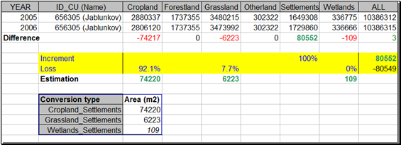
The above described calculation of land-use change could only be performed for the years 1993 to 2010, because the data on land-use for the individual cadastral units has only been available since 1992. For the years preceding 1993, i.e., for land-use change attributed to the years 1970 to 1992, an identical approach as described above was used, but with aggregated cadastral input data at the level on the individual districts. The effect of an increased scale and data aggregation always results in a lower area of identified land-use change. This is probably due to within-domain compensation of area losses and increments. To compensate this effect for the 1970 to 1992 data series, a correction was applied to the estimates, based on district data input. The correction was based on a linear regression function between R (the ratio of identified land conversions at the level of the districts and individual cadastral units) and the logarithmically transformed areas from the data at the district level. The corrections were derived at the level of the major land-use categories, using the annual data from the period of 1993 to 2006, for which the land-use conversions could be estimated independently at both spatial levels, i.e., districts and individual cadastral units. More details, including the statistics and estimated parameters of the regression equation, are given in Cienciala and Apltauer (2007). The correction procedure was the final step in land-use database operations required to provide a consistent data-series on annual land-use conversions for the 1970 to 2010 period.

7.2.2 Land-use change – overall trends and annual matrices

The overall trends in the areas of the major land-use categories in the Czech Republic for the 1970 to 2010 period are shown in Fig 7.4. The largest quantitative change is associated with the Cropland and Grassland land-use categories.

Fig. 7.4 Trends in areas of the six major land-use categories in the Czech Republic between 1970 and 2010 (based on information from the Czech Office for Surveying, Mapping and Cadastre).

An insight into the net trends shown in Fig. 7.4 is provided by analysis of land-use changes as described in Section 7.1.2. Tab. 7.3 shows a product of that analysis, namely the areas of land-use change among the major land-use categories over the 1990 to 2010 period in the form of land-use change matrices for the individual years. It is important to note that the annual totals for the individual years in the matrices do not necessarily correspond to the areas that appear in the CRF Tables, which accounts for the progressing 20-year transition period that began in 1970. This is a Tier 1 assumption of GPG for LULUCF for estimation of changes in soil carbon stock. This also implies that the areas relevant to the biomass pool are not the same as those for the soil pools; this is important for interpretation of the emission factors estimated from the land-use change areas accumulated over 20-year periods. Secondly, for Forest Land, the available input information at a detailed (cadastral, district) level did not permit separation of the fraction of permanently unstocked Forest Land devoted to use other than growing forests. This small fraction of Forest Land was separated ex-post after estimating land-use changes and summing over the whole country, when it was assigned to Grassland.

Tab. 7.3 Land-use matrices describing initial and final areas of particular land-use categories and the identified annual land-use conversions among these categories for years 1990 to 2010.

Year 1990		Initial (1989)						Area (kha)
	Category	Forest Land	Grassland	Cropland	Wetlands	Settlements	Other Land	Area (kha)
Final (1990)	Forest Land	2 628.2	0.5	0.7	0.0	0.0	0.0	2 629.5
	Grassland	0.1	867.3	10.8	0.0	0.0	0.0	878.2
	Cropland	0.1	1.2	3 453.4	0.1	0.2	0.0	3 455.0
	Wetland	0.0	0.4	0.4	155.9	0.8	0.0	157.5
	Settlements	0.3	3.7	3.7	0.1	651.2	0.0	658.9
	Other Land	0.0	0.0	0.0	0.0	0.0	107.2	107.2
	Area (kha)	2 628.7	873.1	3 469.0	156.1	652.2	107.2	7 886.4

Year 1991		Initial (1990)						Area (kha)
	Category	Forest Land	Grassland	Cropland	Wetlands	Settlements	Other Land	Area (kha)
Final (1991)	Forest Land	2 628.8	0.1	0.4	0.0	0.0	0.0	2 629.3
	Grassland	0.4	876.4	32.6	0.0	0.3	0.0	909.8
	Cropland	0.3	0.5	3 419.4	0.0	0.2	0.0	3 420.4
	Wetland	0.1	0.1	0.6	157.4	0.0	0.0	158.1
	Settlements	0.2	0.3	3.4	0.0	657.7	0.0	661.6
	Other Land	0.0	0.0	0.0	0.0	0.0	107.2	107.2
	Area (kha)	2 629.6	877.4	3 456.4	157.4	658.2	107.2	7 886.4

Year 1992		Initial (1991)						Area (kha)
	Category	Forest Land	Grassland	Cropland	Wetlands	Settlements	Other Land	Area (kha)
Final (1992)	Forest Land	2 628.7	0.1	0.2	0.0	0.0	0.0	2 629.1
	Grassland	0.2	907.3	10.2	0.1	0.0	0.0	917.9
	Cropland	0.1	0.7	3 409.9	0.0	0.2	0.0	3 410.9
	Wetland	0.0	0.1	0.2	157.8	0.0	0.0	158.1
	Settlements	0.3	0.4	2.0	0.1	660.5	0.0	663.3
	Other Land	0.0	0.0	0.0	0.0	0.0	107.2	107.2
	Area (kha)	2 629.5	908.6	3 422.4	158.0	660.7	107.2	7 886.4

Year 1993		Initial (1992)						Area (kha)
	Category	Forest Land	Grassland	Cropland	Wetlands	Settlements	Other Land	Area (kha)
Final (1993)	Forest Land	2 628.2	0.1	0.1	0.0	0.2	0.0	2 628.6
	Grassland	0.1	916.6	1.6	0.0	0.3	0.0	918.6
	Cropland	0.2	0.6	3 407.9	0.0	0.4	0.0	3 409.1
	Wetland	0.0	0.1	0.0	157.9	0.3	0.0	158.3
	Settlements	0.5	0.4	1.2	0.1	662.3	0.0	664.6
	Other Land	0.0	0.0	0.0	0.0	0.0	107.2	107.2
	Area (kha)	2 629.1	917.8	3 410.9	158.1	663.4	107.2	7 886.4

Year 1994		Initial (1993)						Area (kha)
	Category	Forest Land	Grassland	Cropland	Wetlands	Settlements	Other Land	Area (kha)
Final (1994)	Forest Land	2 628.1	0.2	0.2	0.1	0.9	0.0	2 629.5
	Grassland	0.1	917.2	14.8	0.0	0.4	0.0	932.5
	Cropland	0.1	0.7	3 392.7	0.0	0.4	0.0	3 394.0
	Wetland	0.0	0.1	0.0	158.1	0.4	0.0	158.6
	Settlements	0.4	0.4	1.3	0.1	662.6	0.0	664.8
	Other Land	0.0	0.0	0.0	0.0	0.0	107.2	107.2
	Area (kha)	2 628.7	918.6	3 409.1	158.4	664.7	107.2	7 886.7

Year 1995		Initial (1994)						Area (kha)
	Category	Forest Land	Grassland	Cropland	Wetlands	Settlements	Other Land	Area (kha)
Final (1995)	Forest Land	2 629.0	0.4	0.3	0.0	0.5	0.0	2 630.1
	Grassland	0.1	930.9	15.4	0.0	0.5	0.0	946.9
	Cropland	0.2	0.8	3 376.9	0.1	0.6	0.0	3 378.5
	Wetland	0.0	0.1	0.1	158.4	0.4	0.0	159.1
	Settlements	0.3	0.4	1.2	0.1	662.8	0.0	664.8
	Other Land	0.0	0.0	0.0	0.0	0.0	107.2	107.2
	Area (kha)	2 629.5	932.5	3 393.9	158.6	664.8	107.2	7 886.6

Year 1996		Initial (1995)						Area (kha)
	Category	Forest Land	Grassland	Cropland	Wetlands	Settlements	Other Land	Area (kha)
Final (1996)	Forest Land	2 629.2	0.4	0.9	0.0	0.5	0.0	2 631.0
	Grassland	0.3	943.7	45.4	0.1	1.3	0.0	990.9
	Cropland	0.2	2.2	3 330.8	0.1	0.8	0.0	3 334.0
	Wetland	0.0	0.1	0.1	158.8	0.3	0.0	159.3
	Settlements	0.4	0.5	1.4	0.1	661.8	0.0	664.2
	Other Land	0.0	0.0	0.0	0.0	0.0	107.2	107.2
	Area (kha)	2 630.1	946.9	3 378.6	159.1	664.7	107.2	7 886.7

Year 1997		Initial (1996)						Area (kha)
	Category	Forest Land	Grassland	Cropland	Wetlands	Settlements	Other Land	Area (kha)
Final (1997)	Forest Land	2 630.1	0.4	0.3	0.0	0.9	0.0	2 631.8
	Grassland	0.2	987.2	10.2	0.1	1.1	0.0	998.8
	Cropland	0.2	2.6	3 322.2	0.1	1.3	0.0	3 326.4
	Wetland	0.0	0.1	0.1	159.0	0.2	0.0	159.4
	Settlements	0.4	0.6	1.1	0.1	660.8	0.0	662.9
	Other Land	0.0	0.0	0.0	0.0	0.0	107.2	107.2
	Area (kha)	2 630.9	990.9	3 334.0	159.3	664.3	107.2	7 886.6

Year 1998		Initial (1997)						Area (kha)
	Category	Forest Land	Grassland	Cropland	Wetlands	Settlements	Other Land	Area (kha)
Final (1998)	Forest Land	2 630.3	0.7	0.5	0.1	2.3	0.0	2 633.8
	Grassland	0.4	983.6	5.8	0.3	2.8	0.0	992.9
	Cropland	0.4	13.4	3 318.3	0.4	4.5	0.0	3 337.0
	Wetland	0.1	0.2	0.1	158.2	0.4	0.0	159.0
	Settlements	0.5	0.9	1.5	0.3	652.9	0.0	656.1
	Other Land	0.0	0.0	0.0	0.0	0.0	107.2	107.2
	Area (kha)	2 631.7	998.8	3 326.2	159.3	662.8	107.2	7 886.0

Year 1999		Initial (1998)						Area (kha)
	Category	Forest Land	Grassland	Cropland	Wetlands	Settlements	Other Land	Area (kha)
Final (1999)	Forest Land	2 632.9	0.5	0.3	0.0	0.7	0.0	2 634.5
	Grassland	0.1	991.1	4.1	0.0	0.4	0.0	995.7
	Cropland	0.1	0.9	3 330.6	0.0	0.6	0.0	3 332.2
	Wetland	0.1	0.1	0.2	158.7	0.1	0.0	159.2
	Settlements	0.6	0.6	1.9	0.1	654.4	0.0	657.5
	Other Land	0.0	0.0	0.0	0.0	0.0	107.2	107.2
	Area (kha)	2 633.8	993.1	3 337.1	159.0	656.2	107.2	7 886.4

Year 2000		Initial (1999)						Area (kha)
	Category	Forest Land	Grassland	Cropland	Wetlands	Settlements	Other Land	Area (kha)
Final (2000)	Forest Land	2 633.8	0.5	0.5	0.1	2.4	0.0	2 637.3
	Grassland	0.1	992.9	13.1	0.1	0.4	0.0	1 006.6
	Cropland	0.1	1.7	3 316.6	0.1	0.3	0.0	3 318.8
	Wetland	0.1	0.1	0.2	158.9	0.1	0.0	159.3
	Settlements	0.4	0.5	1.9	0.1	654.3	0.0	657.2
	Other Land	0.0	0.0	0.0	0.0	0.0	107.2	107.2
	Area (kha)	2 634.5	995.8	3 332.2	159.3	657.5	107.2	7 886.5

Year 2001		Initial (2000)						Area (kha)
	Category	Forest Land	Grassland	Cropland	Wetlands	Settlements	Other Land	Area (kha)
Final (2001)	Forest Land	2 636.8	0.5	0.4	0.0	1.1	0.0	2 638.9
	Grassland	0.1	1 004.8	6.0	0.0	0.5	0.0	1 011.4
	Cropland	0.1	0.8	3 310.3	0.0	0.3	0.0	3 311.6
	Wetland	0.0	0.1	0.1	159.2	0.1	0.0	159.6
	Settlements	0.3	0.4	1.9	0.1	655.1	0.0	657.8
	Other Land	0.0	0.0	0.0	0.0	0.0	107.2	107.2
	Area (kha)	2 637.3	1 006.6	3 318.7	159.4	657.2	107.2	7 886.5

Year 2002		Initial (2001)						Area (kha)
	Category	Forest Land	Grassland	Cropland	Wetlands	Settlements	Other Land	Area (kha)
Final (2002)	Forest Land	2 638.4	0.9	1.1	0.0	2.5	0.0	2 643.1
	Grassland	0.1	1 009.3	3.7	0.0	0.9	0.0	1 014.0
	Cropland	0.0	0.3	3 303.9	0.1	0.1	0.0	3 304.5
	Wetland	0.1	0.1	0.2	159.4	0.2	0.0	159.9
	Settlements	0.3	0.8	2.6	0.1	654.3	0.0	658.1
	Other Land	0.0	0.0	0.0	0.0	0.0	107.2	107.2
	Area (kha)	2 638.9	1 011.4	3 311.6	159.6	658.0	107.2	7 886.8

Year 2003		Initial (2002)						Area (kha)
	Category	Forest Land	Grassland	Cropland	Wetlands	Settlements	Other Land	Area (kha)
Final (2003)	Forest Land	2 642.1	0.6	0.7	0.0	0.7	0.0	2 644.2
	Grassland	0.1	1 011.2	4.6	0.0	0.3	0.0	1 016.3
	Cropland	0.1	1.5	3 296.9	0.0	0.1	0.0	3 298.6
	Wetland	0.0	0.1	0.2	159.7	0.1	0.0	160.1
	Settlements	0.5	0.6	2.1	0.1	656.9	0.0	660.2
	Other Land	0.0	0.0	0.0	0.0	0.0	107.2	107.2
	Area (kha)	2 642.9	1 014.0	3 304.5	159.9	658.1	107.2	7 886.7

Year 2004		Initial (2003)						Area (kha)
	Category	Forest Land	Grassland	Cropland	Wetlands	Settlements	Other Land	Area (kha)
Final (2004)	Forest Land	2 643.5	0.8	0.8	0.0	0.6	0.0	2 645.7
	Grassland	0.1	1 013.8	3.1	0.0	0.4	0.0	1 017.4
	Cropland	0.1	0.7	3 291.9	0.0	0.2	0.0	3 292.8
	Wetland	0.0	0.2	0.2	159.9	0.1	0.0	160.5
	Settlements	0.5	0.9	2.7	0.1	658.9	0.0	663.1
	Other Land	0.0	0.0	0.0	0.0	0.0	107.2	107.2
	Area (kha)	2 644.2	1 016.4	3 298.7	160.1	660.2	107.2	7 886.8

Year 2005		Initial (2004)						Area (kha)
	Category	Forest Land	Grassland	Cropland	Wetlands	Settlements	Other Land	Area (kha)
Final (2005)	Forest Land	2 645.1	0.9	0.9	0.0	0.6	0.0	2 647.4
	Grassland	0.1	1 015.1	4.0	0.0	0.3	0.0	1 019.5
	Cropland	0.1	0.4	3 284.9	0.0	0.2	0.0	3 285.7
	Wetland	0.0	0.2	0.2	160.4	0.1	0.0	160.9
	Settlements	0.4	0.8	2.7	0.1	661.9	0.0	666.0
	Other Land	0.0	0.0	0.0	0.0	0.0	107.2	107.2
	Area (kha)	2 645.7	1 017.4	3 292.8	160.5	663.1	107.2	7 886.7

Year 2006		Initial (2005)						Area (kha)
	Category	Forest Land	Grassland	Cropland	Wetlands	Settlements	Other Land	Area (kha)
Final (2006)	Forest Land	2 647.0	0.7	1.0	0.0	0.4	0.0	2 649.1
	Grassland	0.1	1 017.6	4.0	0.0	0.2	0.0	1 021.9
	Cropland	0.1	0.4	3 277.5	0.0	0.2	0.0	3 278.2
	Wetland	0.0	0.2	0.3	160.7	0.2	0.0	161.4
	Settlements	0.3	0.7	2.8	0.1	664.9	0.0	668.8
	Other Land	0.0	0.0	0.0	0.0	0.0	107.2	107.2
	Area (kha)	2 647.4	1 019.5	3 285.6	160.9	665.9	107.2	7 886.7

Year 2007		Initial (2006)						Area (kha)
	Category	Forest Land	Grassland	Cropland	Wetlands	Settlements	Other Land	Area (kha)
Final (2007)	Forest Land	2 648.8	0.6	0.9	0.0	0.9	0.0	2 651.2
	Grassland	0.1	1 019.9	3.5	0.0	0.2	0.0	1 023.7
	Cropland	0.0	0.5	3 270.4	0.0	0.2	0.0	3 271.2
	Wetland	0.0	0.2	0.3	161.2	0.4	0.0	162.1
	Settlements	0.3	0.7	3.0	0.1	667.1	0.0	671.2
	Other Land	0.0	0.0	0.0	0.0	0.0	107.2	107.2
	Area (kha)	2 649.1	1 021.9	3 278.1	161.4	668.8	107.2	7 886.7

Year 2008		Initial (2007)						Area (kha)
	Category	Forest Land	Grassland	Cropland	Wetlands	Settlements	Other Land	Area (kha)
Final (2008)	Forest Land	2 650.8	0.5	0.8	0.1	0.9	0.0	2 653.0
	Grassland	0.0	1 021.8	3.3	0.0	0.1	0.0	1 025.4
	Cropland	0.1	0.4	3 263.6	0.0	0.2	0.0	3 264.4
	Wetland	0.0	0.2	0.3	161.9	0.1	0.0	162.5
	Settlements	0.3	0.7	3.1	0.1	669.8	0.0	674.0
	Other Land	0.0	0.0	0.0	0.0	0.0	107.2	107.2
	Area (kha)	2 651.2	1 023.6	3 271.1	162.1	671.2	107.2	7 886.5

Year 2009		Initial (2008)						Area (kha)
	Category	Forest Land	Grassland	Cropland	Wetlands	Settlements	Other Land	Area (kha)
Final (2009)	Forest Land	2 652.6	0.7	0.8	0.1	1.1	0.0	2 655.2
	Grassland	0.1	1 023.3	4.7	0.0	0.3	0.0	1 028.4
	Cropland	0.0	0.5	3 255.4	0.0	0.2	0.0	3 256.2
	Wetland	0.0	0.2	0.3	162.9	0.1	0.0	162.8
	Settlements	0.3	0.8	3.2	0.2	672.2	0.0	676.6
	Other Land	0.0	0.0	0.0	0.0	0.0	107.2	107.2
	Area (kha)	2 653.0	1 025.4	3 264.3	162.5	674.0	107.2	7 886.5

Year 2010		Initial (2009)						Area (kha)
	Category	Forest Land	Grassland	Cropland	Wetlands	Settlements	Other Land	Area (kha)
Final (2010)	Forest Land	2 654.6	0.6	1.1	0.1	0.9	0.0	2 657.4
	Grassland	0.1	1 026.1	4.8	0.0	0.5	0.0	1 031.5
	Cropland	0.1	0.6	3 246.7	0.0	0.2	0.0	3 247.6
	Wetland	0.1	0.2	0.4	162.3	0.2	0.0	163.1
	Settlements	0.3	1.0	3.2	0.3	674.7	0.0	679.6
	Other Land	0.0	0.0	0.0	0.0	0.0	107.2	107.2
	Area (kha)	2 655.2	1 028.5	3 256.2	162.8	676.6	107.2	7 886.5

7.2.3 Methodologies to estimate emissions

The estimation of emissions and removals of CO₂ and non-CO₂ gases for the sector was performed according to Chapter 3 of GPG for LULUCF (IPCC 2003). Additionally, the 2006 Guidelines for National Greenhouse Gas Inventories – Agriculture, Forestry and Other Land Use (IPCC 2006) were consulted whenever appropriate. The following text describes the inventory for the individual land-use categories, noting vital information on the category within the conditions of the Czech Republic, the methodology employed, uncertainty and time consistency, QA/QC and verification, recalculations and source-specific planned improvements.

7.3 Forest Land (5A)

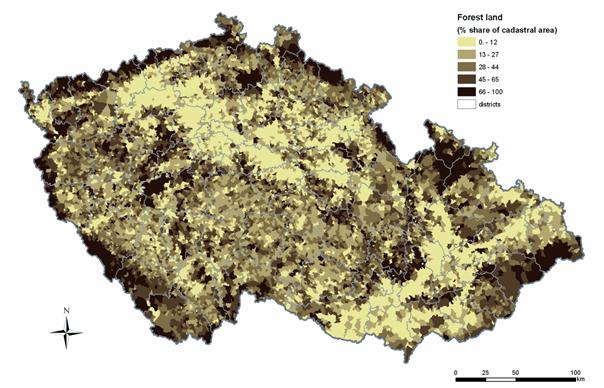
Fig. 7.5 Forest Land in the Czech Republic –distribution calculated as a spatial share of the category within individual cadastral units (as of 2010).

7.3.1 Source category description

The Czech Republic is a country with a long forestry tradition. Practically all the forests can be considered to be temperate-zone managed forests under the IPCC definition of forest management (GPG Chapter 3, IPCC 2003). With respect to the definition thresholds of the Marrakesh Accords, Forest Land is defined as land with woody vegetation and with tree crown cover of at least 30 %, over an area exceeding 0.05 ha containing trees able to reach a minimum height of 2 m at maturity[16]. This definition of forests excludes the areas of permanently unstocked cadastral forest land, such as forest roads, forest nurseries and land under power transmission lines. The permanently unstocked area of cadastral forest land has predominantly the attributes of Grassland, and therefore it was ascribed to that category. Hence, Forest Land in this emission inventory corresponds to the national definition of timberland (Czech Forestry Act 84/1996). In 2010, the stocked forest area (timberland) qualifying under the category of Forest Land in this emission inventory equaled 2 604 thousand ha, representing 98 % of the cadastral forest land in the Czech Republic. The permanently unstocked area represents 2 % of the forest land according to cadastral data and it was linked by this proportion to the area of Forest Land for the whole time series since 1969.

Forests (cadastral forest land) currently occupy 33.7 % of the area of the country (MA 2011). The tree species composition is dominated by conifers, which represent 73.9 % of the timberland area. The four most important tree species in this country are spruce, pine, beech and oak, which account for 51.9, 16.8, 7.3 and 6.9 % of the timberland area, respectively (MA 2011). Broadleaved tree species have been favored in new afforestation since 1990. The proportion of broadleaved tree species increased from 21 % in 1990 to about 25 % in 2010. The total growing stock (merchantable wood volume) in forests in the country has increased during the reported period from 564 mil. m³ in 1990 to 681 mil. m³ (under bark) in 2010 (MA 2011).

Several sources of information on forests are available in the Czech Republic. The primary source of activity data on forests used for this emission inventory is the forest taxation data in Forest Management Plans (further denoted as FMP), which are administered centrally by the Forest Management Institute (FMI), Brandýs n. L. With a forest management plan cycle of 10 years, the annual update of the FMP database is related to 1/10 of the total forest area scattered throughout the country. The information in FMP represents an ongoing national stand-wise type of forest inventory. The second source of information consists in the data from the first cycle of the statistical (sample based, tree level) forest inventory performed during 2001-2004 by FMI. The results of this forest inventory were published in 2007 (FMI, 2007)[17]. The most recent statistical information on forests at a county level gives the Czech landscape inventory (CzechTerra; www.czechterra.cz), a project funded by the Ministry of Environment (Černý 2009, SP/2d1/93/07)[18]. This emission inventory is dominantly based on the FMP data, which have also been used for all the international reporting on forests of the Czech Republic to date. Whenever feasible, the information from other inventory programs mentioned above and/or other sources was also utilized.

FMP data were aggregated in line with the country-specific approaches at the level of the four major tree species (i-beech: all broadleaved species except oaks, ii-oak: all oak species, iii-pine: pines and larch, iv-spruce: all conifers except pines and larch) and age-classes (10-year intervals). For these categories, growing stock (merchantable volume, defined as tree stem and branch volume under bark with a minimum diameter threshold of 7 cm), the corresponding areas and other auxiliary information were available for each inventory year. It can be observed in Fig. 7.6 that the average growing stock has increased steadily for all tree species groups since 1990 in this country. In addition to the four major categories by predominant tree species, clear-cut areas are also distinguished, forming another, specific sub-category of Forest Land as reported in this submission. A clear-cut area is defined as a temporarily unstocked area following final or salvage harvest of forest stands. It ceases to exist once it is reforested, which must occur within two years according to the Czech Forestry Act. There is no detectable carbon stock change for this category and it is introduced solely for the purpose of consolidated, transparent and consistent reporting of forest land. In 2010, clear-cut areas represented 1.1 % of Forest Land.

Fig. 7.6 Activity data – mean growing stock volume against stand age for the four major groups of species during 1990 to 2010; each line corresponds to an individual inventory year. The symbols identify only the situation in 1990 and 2010.

The annual harvest volume constitutes the other key information related to forestry. This value is available from the Czech Statistical Office (CzSO). CzSO collects this information on the basis of about 600 country respondents (relevant forest companies and forest owners) and encompasses commercial harvest and fuel wood, and included compensation for the forest areas not covered by the respondents. The total drain of merchantable wood from forests increased from 13.3 mil. m³ in 1990 to 16.7 mil. m³ in 2010, down from the all-time high 18.5 mil. m³ harvested in 2007 (all data refer to underbark volumes, MA 2011). Additionally in the emission inventory, harvest loss of 5 and 15 % is applied to final and salvage logging volumes, respectively (see Section 7.3.2 below). The salvage logging operations concern primarily stands of coniferous species, which are commonly hit by windstorms, snow and bark-beetle calamities in this country.

7.3.2 Methodological aspects

Category 5A Forest Land includes emissions and sinks of CO₂ associated with forests and non-CO₂ gases generated by burning in forests. This category is composed of 5A1 Forest Land remaining Forest Land, and 5A2 Land converted to Forest Land. The following text describes the major methodological aspects related to emission inventories of both forest sub-categories.

The methods of area identification described in Section 7.1.2 distinguish the areas of forest with no land-use change over the 20 years prior the reporting year. These lands are included in subcategory 5A1 Forest Land remaining Forest Land. The other part represents subcategory 5A2 Land converted to Forest Land, i.e., the forest areas “in transition” that were converted from other land-use categories over the 20 years prior to the reporting year. The areas of forest subcategories, i.e., 5A1 and 5A2 accumulated over a 20-year rolling period can be found in the corresponding CRF Tables. The annual matrices of identified land-use and land-use changes are given in Tab. 7.3 above.

7.3.2.1 Forest Land remaining Forest Land

Carbon stock change in category 5A1 Forest Land remaining Forest Land is given by the sum of changes in living biomass, dead organic matter and soils. The carbon stock change in living biomass was estimated using the default method[19] according to Eq. 3.3.2 of GPG for LULUCF. This method is based on separate estimation of increments and removals, and their difference.

The reported growing stock of merchantable volume from the database of FMP formed the basis for assessment of the carbon increment (Eqs. 3.2.4 and 3.2.5 of GPG for LULUCF). The key input to calculate the carbon increment is the volume increment (I_v) data. In the Czech Republic, these values have been traditionally calculated by FMI (FMP database administrator; see also Acknowledgment) and reported to the national and international statistics. The calculation is performed at the level of the individual stands and species using the available growth and yield data and models. The increment data were partly revised in the earlier NIR (2008) to unify two different base information sources (Schwappach 1923; Černý et al. 1996) for increment estimates and to apply only the latest source across the entire reporting period. This was to comply with the GPG for LULUCF requirements of consistent time series. No change, apart from entering the increment of latest reported year, was made to the increment in the inventory submissions thereafter (Fig. 7.7).

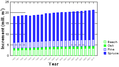
Fig. 7.7 Current annual increment (I_V; m³ underbark) by the individual tree species groups as used in the reporting period 1990 to 2010.

The merchantable volume increment (I_v) is converted to the biomass increment (G_Total), biomass conversion and expansion factors applicable for increment (BCEF_i) using Eqs. 2.9 and 2.10 (AFOLU 2006) as follows:

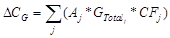
(1)

where A_jand CF_jrepresent the actual stand area (ha) and carbon fraction of dry matter (t C per t dry matter), respectively, for each major tree species type j (beech, oak, pine, spruce), while is calculated for each j as follows:

(2)

where R is a root/shoot ratio to include the below-ground component. The total biomass increment is multiplied by the carbon fraction and the applicable forest land area. Tab. 7.4 lists the factors used in the calculation of the biomass carbon stock increment.

Tab. 7.4 Input data and factors used in carbon stock increment calculation (1990 and 2010 shown) for beech, oak, pine and spruce species groups, respectively.

Variable or conversion factor	Unit	Year 1990	Year 2010
Area of forest land remaining forest land (A)	kha	372; 152; 455; 1504	466; 176; 431; 1462
*Biomass conv. & exp. factor, incr. (BCEF_i)*	Mg m^-3	0.74; 0.86; 0.52; 0.60	0.74; 0.85; 0.53; 0.60
Carbon fraction in biomass (CF)	t C/t biomass	0.50	0.50
Root/shoot ratio (R)	-	0.20	0.20
*Volume increment (I_v)*	m³	6.55; 5.96; 5.84; 7.89	7.14; 6.23; 6.81; 9.31

In Tab. 7.4, A represents only the areas of 5A1 Forest Land remaining Forest Land, updated annually. The applied biomass conversion and expansion factors applicable for the increment (BCEF_i) and growing stock volumes (BCEF_h) are based on national allometric studies (Cienciala et al. 2006a, 2006b, 2008a) or biomass compilations that include data from the Czech Republic (Wirth et al. 2004, Wutzler et al. 2008). Since the biomass conversion and expansion factors are age-dependent (Lehtonen et al. 2004, 2007), they respect the actual age-class distribution of the dominant tree species. Hence, the BCEF_i values shown in Table 7.4 are weighted means considering the actual volumes of the individual age classes for each of the major tree species. Besides the allometric equations noted above, the source dendrometrical material used for derivation of the country-specific BCEF_i values were the data of the landscape inventory program CzechTerra (Černý 2009). Its first cycle was completed in 2009 and these dendrometrical data hence represent the most current information on the Czech Forests available in the country. The tree level data together with the information of age was used to assess the median BCEF_i values for each age class and major tree species. CF of 0.50 is a generally accepted default constant, which is also recommended by IPCC (2003). R was selected as a conservative value from the range recommended for temperate-zone forests by IPCC (2003). It corresponds well to the available relevant experimental evidence (Černý 1990, Green et al. 2006), as well as to the evidence apparent from the parameterized allometric equations for the major tree species (Wirth et al. 2004, Wutzler et al. 2008). I_v is the annually updated volume increment estimated per hectare and species group as described above.

The estimation of carbon drain (L; Eq. 2) in the category 5A1 Forest Land remaining Forest Land basically follows Eqs. 3.2.6, 3.2.7 and 3.2.8 (IPCC 2003). It uses the annual amount of total harvest removals (H) reported by the CzSO for individual tree species in the country. H covers thinning and final cut, as well as the amount of fuel wood, which is reported as an assortment under the conditions of Czech Forestry. To include a potentially unaccounted-for loss associated with H, the factor F_HL was applied to H; it was calculated from annual harvest data and the share of salvage logging, assuming 5 % loss under planned forest harvest operations and 15 % for accidental/salvage harvest applicable for coniferous species. Hence, the harvest volumes entering the actual emission calculation (H in eq. 3 below) include the correction by the above described factor, F_HL. The calculation of the carbon drain (L; loss of carbon) otherwise also follows Eq. 2.12 (AFOLU 2006) as

(3)

where BCEF_h represents a biomass expansion and conversion factor applicable to harvested volumes, derived from national studies or regional compilations that include the data from the Czech Republic as noted and mentioned above. The application of BCEF_h considers the share of the planned harvested volume and the actual salvage logging that was not planned. In the case of planned harvest volumes, the age-dependent BCEF_h values also consider the mean felling age, which is taken from the national reports of the Ministry of Agriculture. For salvage logging, BCEF_h represents the volume-weighted mean of all age classes for the individual dominant tree species, as the actual stand age of those harvested volumes is unknown. The other factors (CF, R) are identical to those described under Tab. 7.4. The specific values of input variables and conversion factors used to calculate L are listed in Table 7.5.

Tab. 7.5 Specific input data and factors used in calculation of carbon drain (1990 and 2010 shown) for beech, oak, pine and spruce species groups, respectively.

Variable or conversion factor	Unit	Year 1990	Year 2010
Harvest volume (H)	mill. m³	0.84; 0.31; 1.33; 10.8	1.28; 0.39; 2.08; 13.0
*Biomass expansion factor (BCEF_h)*	Mg m^-3	0.69; 0.81; 0.52; 0.59	0.69; 0.81; 0.52; 0.58

The impact of disturbances (Eq. 2.14, AFOLU 2006) has not been explicitly estimated. To the present time, the disturbance in Czech forests since 1990 has not reached proportions above the buffering capacity of Czech forestry management practices. Consequently, any salvage felling is flexibly allocated to the desired amount of planned wood removals, and is thereby accounted for in the reported harvest volumes.

The assessment of the net carbon stock change in organic matter (deadwood and litter) followed the Tier 1 (default) GPG for LULUCF assumption of zero change in these carbon pools. This is a safe assumption, as the country did not experience significant changes in forest types, disturbance or management regimes within the reporting period.

The above assumption also applies to the soil carbon pool, in which the net carbon stock change was considered to equal zero (Tier 1, IPCC 2003). This concerns both mineral and organic soils. The organic soils occur only in the areas of the Spruce sub-category on 5A1 Forest Land remaining Forest Land. They represent protected peat areas in mountainous regions dominated by spruce stands, with no or specific management practices. No such areas occur under other the sub-categories by the predominant species of Beech, Oak and Pine.

Emissions in category 5A1 Forest Land remaining Forest Land include, in addition to CO₂, also other greenhouse gases (CH₄, CO, N₂O and NO_x) resulting from burning. This encompasses both prescribed fires associated with burning of biomass residues and also emissions due to wildfires. The emissions from burning of biomass residues were estimated according to Eq. 3.2.19 and the emission ratios in Table 3A.1.15 (Tier 1, IPCC 2003). Under the conditions in this country, part of the biomass residues is burned in connection with final cut. The expert judgment employed in this inventory revision considers that 30 % of the biomass residues including bark is burned. This biomass fraction was quantified on the basis of the annually reported amount of final felling volume of broadleaved and coniferous species, BCEF_h and CF as applied to harvest removals (above). The amount of biomass burned (dry matter) was estimated as 585 Gg in 1990 and 748 Gg in 2010.

The emissions of greenhouse gases due to wildfires were estimated on the basis of known areas burnt annually by forest fires and the average biomass stock in forests according to Eq. 3.2.9 (IPCC 2003). This equation used a default factor of biomass left to decay after burning (0.45; Table 3A.1.12). The associated amounts of non-CO₂ gases (CH₄, CO, N₂O and NO_x) were estimated according to Eq. 3.2.19. The amount of biomass (dry matter) burned in wildfires was estimated as 10.2 Gg in 1990 and 15.1 Gg in 2010. The most extreme year of the reporting period was 1997, when about 228 Gg of biomass was burned due to wildfires. The full time series and the associated emissions of non-CO₂ gases can be found in the corresponding CRF tables.

There are no direct N₂O emissions from N fertilization on Forest Land, as there is no practice of nitrogen fertilization of forest stands in the Czech Republic. Similarly, non-CO₂ emissions related to drainage of wet forest soils are not reported, as this activity no longer occurs in practice.

7.3.2.2 Land converted to Forest Land

The methods employed to estimate emissions in the 5A2 Land converted to Forest Land category are similar to those for the category of Forest Land remaining Forest Land, but they differ in some assumptions, which follow the recommendations of GPG for LULUCF.

For estimation of the net carbon stock change in living biomass on Land converted to Forest Land by the Tier 1 method (IPCC 2003), the carbon increment is proportional to the extent of afforested areas and the growth of biomass. The revised methodology of land-use change identification (Section 7.1.2) provides areas of all conversion types updated annually. Land areas are considered to be under conversion for a period of 20 years, according the Tier 1 assumption of GPG for LULUCF. Under the conditions in this country, all newly afforested lands are considered as intensively managed lands under the prescribed forest management rules as specified by the Czech Forestry Act.

Until 2006, the increment applicable to age classes I and II (stand age up to 20 years) was estimated from the actual wood volumes and areas that were available per major species groups. Using the available activity stand level data categorized by species and age classes and the national growth and yield model SILVISIM (Černý 2005), the wood increment was derived for all the age classes above 20 years. For age class one (1-10 years), the increment was simply calculated from the reported areas and volumes, assuming a mean age of five years. The increment of age class two (11 to 20 years) was estimated from linear interpolation between the increment of age classes I and III. For the year 2007 and forward, increment is derived for individual tree species using the ratio of increment for individual tree species to the total stand increment estimated from the period 2000 to 2006.

Since the specific species composition of the newly converted land is unknown, the increment estimated for the major tree species was averaged using the weight of actual areas for the individual tree species known from the unchanged (remaining) forest land. Expressed in terms of aboveground biomass, the estimated aggregated mean increment for 2010 was 3.15 t/ha, a value matching that for temperate coniferous (3 t/ha) and somewhat lower than that for broadleaved (4 t/ha) forests given as defaults in GPG for LULUCF. The estimation of increment in terms of aboveground biomass is facilitated by the age and species dependent BCEF_i values as described in Section 7.3.2.1 above. The estimated species-specific values of BCEF_i applicable for young trees until 20 years were 0.99, 1.25, 0.65 and 0.93 for beech, oak, pine and spruce, respectively.

The carbon loss associated with biomass in the category of Land converted to Forest Land was assumed to be insignificant (zero). This is because the first significant thinning occurs in older age classes, which is implicitly accounted for within the category Forest Land remaining Forest Land.

The net changes of carbon stock in dead organic matter were assumed to be insignificant (zero), in accordance with the assumptions of the Tier 1 method (IPCC 2003).

The net change of carbon stock in mineral soils was estimated using the country-specific Tier 2/Tier 3 method. It was based on the vector map of topsoil organic carbon content (Macků et al. 2007, Šefrna and Janderková 2007; Fig. 7.8). The map constructed for forest soils utilized over six thousand soil samples, linking the forest ecosystem units - stand site types and ecological series available in maps 1:5 000 and 1:10 000, as used in the Czech system of forest typology (Macků et al. 2007). This represents the soil organic carbon content to a reference depth of 30 cm, including the upper organic horizon. The carbon content on agricultural soils was prepared so as to match the forest soil map in terms of reference depth and categories of carbon content, although based on interpretation of coarser 1:50 000 and 1:500 000 soil maps (Šefrna and Janderková 2007). The polygonal source maps were used to obtain the mean carbon content per individual cadastral unit (n=12 959 in 2010), serving as reference levels of soil carbon stock applicable to forest and agricultural soils. Since agricultural soils include both Cropland and Grassland land-use categories, the bulk soil carbon content obtained from the map was adjusted for the two categories. This was performed by applying a ratio of 0.85 relating the soil carbon content between Cropland and Grassland (J. Šefrna, personal communication 2007) and considering the actual areas of Cropland and Grassland in the individual cadastral units. This system permitted estimation of the soil carbon stock change among categories 5A Forest Land, 5B Cropland and 5C Grassland. The estimated quantities of carbon stock change at the level of the individual spatial units entered 20-year accumulation matrices distributing carbon into fractions over 20 years (Tier 1, IPCC 2003). These quantities, together with the accumulated areas under the specific conversion categories, were used for estimation of emissions and removals of CO₂.

The net changes of carbon stock in organic soils, occurring only in the sub-category of stands dominated by spruce, were assumed to be insignificant (zero). This is in accordance with the general assumption of the Tier 1 method applicable for forest soils, as no other specific methodology is available for organic soils besides the drained ones (IPCC 2003).

Non-CO₂ emissions from burning are not estimated for category 5A2 Land converted to Forest Land, as there is no such practice in this country. The same applies to the N₂O emissions from nitrogen fertilization, which is not employed in this country.

Fig. 7.8 Top - topsoil (30 cm) organic carbon content map adapted from Macků et al. (2007), Šefrna and Janderková (2007); bottom –topsoil carbon content for agricultural (left) and forest (right) soils estimated as cadastral unit means from the source maps. The unit (t/ha) and unit categories are identical for all maps.

7.3.3 Uncertainty and time consistency

The methods used in this inventory were consistently employed across the whole reporting period from the base year of 1990 to 2010.

The uncertainty estimation was guided by the Tier 1 methods outlined in GPG for LULUCF (IPCC 2003), employing the following equations:

(4)

where U_total is the percentage uncertainty in the product of the quantities and U_i denotes the percentage uncertainties with each of the quantities (Eq. 5.2.1, IPCC 2003).

For the quantities that are combined by addition or subtraction, we used the following equation to estimate the uncertainty:

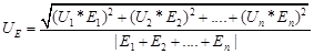
(5)

where U_E is the percentage uncertainty of the sum, U_i is the percentage uncertainty associated with source/sink i, and E_i is the emission/removal estimate for source/sink i (Eq. 5.2.2, IPCC 2003).

It should be noted, however, that Eq. 5 as exemplified in GPG for LULUCF, is not well applicable for the LULUCF sector. Summing negative (removals) and positive (emission) members (E_i) in denominator of Eq. 5 may easily produce unrealistically high uncertainties and theoretically lead to a division by zero, which is not possible. In this respect, this approach is not correct. In previous inventory reports, we stressed this issue and recommended focusing to individual uncertainty components prior the resulting product of Eq. 5.

In this inventory report, we followed the recommendations of the recent reviews and revised the uncertainty values and calculation. The currently adopted uncertainty values are listed below and/or under the corresponding subchapters of other land use categories. Apart the IPCC (2006), the source information for adjusted uncertainty values was the recently conducted statistical landscape inventory of the Czech Republic CzechTerra (Černý et al. 2009). Otherwise, the uncertainty estimation utilized primarily the default uncertainty values as recommended by UNFCCC (2005) and IPCC (2003, 2006) that concern areas of land use (3 %), biomass increment (6 %), amount of harvest (20 %), carbon fraction in dry wood mass (7 %), root/shoot factor (30 %), and factor (1-f_BL; 75 %), used in calculation of emissions from forest fires. The uncertainty applicable to BCEF was 22 %, which was derived from the work of Lehtonen et al. (2007). The uncertainty associated with fractions of unregistered loss of biomass under felling operations was set by expert judgment at 30 %.

Secondly, we revised the approach of uncertainty combination for individual sub-categories of tree species differently in this submission. Specifically, we calculate mean error estimate from the components of carbon stock increase and carbon stock loss, which are both given in identical mass units of carbon per year. At the same time, we preserve the recommended logics of combining uncertainties on the level of entire land use category or on the level of entire LULUCF sector according Eq. 5. This is calculated on the basis of CO₂ or CO₂ eq. units and the corresponding uncertainty estimates respect the actual direction of source and sink categories to be combined. This approach together with the revised emission estimates significantly reduced the overall uncertainty estimates on the level of major land use categories and entire LULUCF sector as compared to previously reported values.

For 2010, the uncertainty estimates for the categories 5A1 Forest Land remaining Forest Land and 5A2 Land converted to Forest Land using the above revised approach reached 25.4 and 38.5 %, respectively. Correspondingly, the uncertainty for the entire category 5A Forest Land reached 25.1 %.

7.3.4 QA/QC and verification

Following the recommendation of the previous in-country review, a sector-specific QA/QC plan was formulated, tightly linked to the corresponding QA/QC plan of the National Inventory System. The plan describes the key procedures of inventory compilation, provides a table of personal responsibilities a timetable of sector-specific QA/QC procedures. This plan consolidates the quality assurance procedures and facilitates an effective quality control of the LULUCF inventory.

Basically all the calculations are based on the activity data taken from the official national sources, such as the Forest Management Institute (Ministry of Agriculture), the Czech Statistical Office, the Czech Office for Surveying, Mapping and Cadastre (COSMC) and the Ministry of the Environment. Data sources are verifiable and updated annually. The gradual development of survey methods and implementation of information technology, checking procedures and increasing demand on quality result in increasing accuracy of the emission estimates. The QA/QC procedures generally cover the elements listed in Table 5.5.1 of GPG for LULUCF (IPCC 2003).

The input information and calculations are archived by the expert team and the coordinator of NIR. Hence, all the background data and calculations are verifiable.

Apart from official review process, emission inventory methods and results are internally reviewed among the technical experts involved in the emission inventory of the Agriculture and LULUCF sectors. Whenever feasible, the methods are subject to peer-review in case of the cited scientific publications, and expert team reviews within the relevant national research projects.

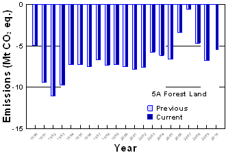
Fig. 7.9 Current and previously reported assessment of emissions for category 5A Forest Land. The values are negative, hence representing net removals of green-house gases.

7.3.5 Recalculations

Since the last submission, no emission recalculation has been performed in the category of Forest Land. Therefore, the current and previous estimates are identical for the jointly reported years (Fig. 7.9).

7.3.6 Source-specific planned improvements

The current revision applicable for Forest Land and associated land-use change introduced improvements regarding uncertainty estimation following the suggestions of the recent inventory reviews. Other recommendations such as reporting emissions/removals by sub-categories of major tree species groups, revised categorization of land-use and an improved land-use determination system were already implemented before. Nonetheless, the category will require additional efforts to further consolidate the estimates. This includes a further improvement of the uncertainty assessment (exploring the Monte-Carlo approaches) and further formalization and enhancement of QA/QC procedures. Over a longer term, utilization of the stock change method in as explored in Cienciala et al. (2006a) will be considered. This involves an assessment of how the data from the recently conducted statistical landscape inventory (CzechTerra, Černý 2009) could be utilized.

Additionally in this inventory, emissions from lime application on forest land is newly included in this submission. These emissions are, however, reported under the category 5G Other due to the current technical limitations of the CRF Reporting software. The addition of emissions from lime application on forest land makes the reporting under Convention compatible with that of KP LULUCF activities where emissions from lime applications are also reported for the activities related to forest land.

7.4 Cropland (5B)

7.4.1 Source category description

In the Czech Republic, Cropland is predominantly represented by arable land (93 % of the category), while the remaining area includes hop-fields, vineyards, gardens and orchards. These categories correspond to five of the six real estate categories on agricultural land from the database of “Aggregate areas of cadastral land categories” (AACLC), collected and administered by COSMC.

Cropland is spatially the largest land-use category in the country. Simultaneously, the area of Cropland has constantly decreased since the 1970s, with a particularly strong decreasing trend since 1990 (Fig. 7.4). While, in 1990, Cropland represented approx. 44 % of the total area of the country, this share decreased to nearly 41 % in 2010. It can be expected that this trend will continue. The conversion of arable land to grassland is also actively promoted by state subsidies. In addition, there is a growing demand for land for infrastructure and settlements. The current estimate of probable excess lands qualifying for conversion to other land-use in the near future is about 600 000 ha. Conversion to grassland concerns mainly the lands of less productive regions of alpine and sub-alpine regions.

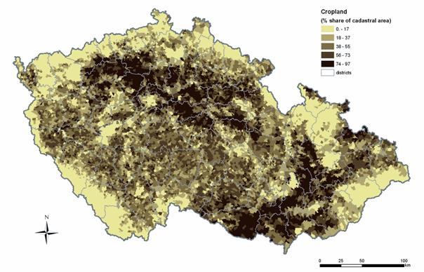
Fig. 7.10 Cropland in the Czech Republic – distribution calculated as a spatial share of the category within individual cadastral units (as of 2010).

7.4.2 Methodological aspects

The emission inventory of Cropland concerns sub-categories 5B1 Cropland remaining Cropland and 5B2 Land converted to Cropland. The emission inventory of Cropland considers changes in living biomass and soil. In addition, CO₂ emissions resulting from application of agricultural limestone and N₂O emissions associated with soil disturbance during land-use conversion to cropland are quantified for this category.

7.4.2.1 Cropland remaining Cropland

For category 5B1 Cropland remaining Cropland, the changes in biomass can be estimated only for perennial woody crops. Under the conditions in this country, this might be applicable to the categories of vineyards, gardens and orchards. Hence, to estimate emissions associated with biomass on Cropland, we applied a default factor for the biomass accumulation rate (2.1 t C/ha/year, Table 3.3.2, IPCC 2003) and estimated changes in the areas concerned.

The carbon stock changes in soil in the category Cropland remaining Cropland are given by changes in mineral and organic soils. Organic soils basically do not occur on Cropland; they occur as peatland in mountainous regions on Forest Land. While organic soils practically do not occur on Cropland, emissions were estimated for mineral soils. Based on the average carbon content on Cropland estimated from the detailed soil carbon maps (Fig. 7.8), we applied the default relative stock change factors for land use (F_LU; 1.0), management (F_MG; 1.08) and input of organic matter (F_I; 1.0), respectively (Table 5.5; IPCC 2006). These differentiate management activities on individual Cropland subcategories, in our case arable land, hop fields and the sub-categories containing perennial woody crops. The average soil carbon on typical arable cropland, estimated as the area-weighted average from individual cadastral units, was 59 t/ha, while it was estimated as 63.7 t/ha for soils with woody vegetation, such as in orchards. The changes in soil carbon stock, associated with the annually changing proportion of land areas of cropland sub-categories, result in emissions/removals. These are calculated after redistribution of the estimated carbon stock change over a 20-year rolling period.

The Cropland category also includes emissions due to liming, which were estimated from the reported limestone use and application area. Liming by either limestone (CaCO₃) or dolomite (CaMg(CO₃)₂) is used to improve soil for crop growth by increasing the availability of nutrients and decreasing acidity. However, the reactions associated with limestone application also lead to evolution of CO₂, which must be quantified. Of the reported total limestone use in agriculture, 95 % was ascribed to Cropland (the reminder to Grassland), based on expert judgment (V. Klement, Central Institute for Supervising and Testing in Agriculture – personal communication, 2005). The quantification followed the Tier 1 method of GPG for LULUCF (Eq. 3.3.6 IPCC 2003), with an emission factor of 0.12 t C/t CaCO₃. Separate data are not available for limestone and dolomite, hence the aggregate estimates for total lime applications are reported.

The application of agricultural limestone was previously intensive in this country, but decreased radically during the 1990s. Hence, the amount of limestone applied in 1990 equaled over 2.5 mil. t, but decreased to less than 200 000 t annually during the most recent years (see the corresponding CRF Tables). This dramatic decrease makes the entire category of 5B1 Cropland remaining Cropland a key category identified by trend, although its quantitative contribution to national emissions in recent years is marginal and reached less than 0.03 % in 2010. The activity data on liming were repeatedly verified. They correspond to the trend reported for use of fertilizers, which decreased a lot in early 1990s (Salusová et. al. 2006).

Non-CO₂ greenhouse gas emissions from burning do not occur in category 5A2 Land converted to Forest Land, as there is no such practice in this country.

7.4.2.2 Land converted to Cropland

Category 5B2 Land converted to Cropland includes land conversions from other land-use categories. Cropland has generally decreased in area since 1990, by far most commonly converted to Grassland. However, the adopted land-use identification system was also able to detect some land conversion in the opposite direction, i.e., to Cropland.

The estimation of carbon stock changes in biomass in the category 5B2 Land converted to Cropland was based on quantifying the difference between the carbon stock before and after the conversion, including the estimate of one year of cropland growth (5 t C/ha; Table. 3.3.8, IPCC 2003), which follows Tier 1 assumptions of GPG for LULUCF and the recommended default values for the temperate zone. For biomass carbon stock on Forest Land prior conversion, the annually updated average growing stock volumes, species-specific volume-weighted biomass conversion and expansion factors ((BCEF), and other factors such as the below-ground biomass ratio were used as described the 5A Forest Land category in Section 7.2.2.1 above. For biomass carbon stock on Grassland prior the conversion, the default factors of 6.8 t/ha for above-ground and below-ground biomass were used (Table 6.4, IPCC 2006). A biomass content of 0 t/ha was assumed after land conversion to 5B Cropland.

The estimation of net carbon stock change in dead organic matter concerns the land use conversion from Forest Land. In this case, the input information on standing and lying deadwood was obtained from the recently (2008 to 2009) conducted field campaign of the Czech landscape inventory CzechTerra (Černý 2009; www.czechterra.cz). It provides data on the mean standing deadwood biomass (2.17 t/ha) and volume of lying deadwood (7.5 m³/ha) classified in four categories according to decomposition degree. These categories are defined as follows: i) basically solid wood; ii) peripheral layers soft, central hard; iii) peripheral layers hard, central soft; iv) totally rotten wood. The amount of carbon held in lying deadwood was estimated as the product of the wood volume, density weighted by mean growing stock volume of major tree species (0.433 t/m³), reduction coefficients of 0.8, 0.5, 0.5, 0.2 (Cerny et al. 2002; Carmona et al. 2002) applicable to the above described decomposition categories, respectively, and the carbon fraction in the wood (0.5 t C/t biomass). A default, conservative assumption that no deadwood is present following the land use change was adopted in this calculation.

The estimation of the carbon stock change in soils for the category 5B2 Land converted to Cropland in the Czech Republic concerns mineral soils. The soil carbon stock changes following the conversion from Forest Land and Grassland were quantified by the country-specific Tier 2/Tier 3 approach is described in detail in Section 7.2.2.2 above.

The Land converted to Cropland category represents a source of non-CO₂ gases, namely emissions of N₂O due to mineralization. The estimation followed the Tier 1 approach of Eqs. 3.3.14 and 3.3.15 (IPCC 2003). Accordingly, N₂O was quantified on the basis of the detected changes in mineral soils employing a default emission factor of 0.0125 kg N₂O-N/kg N, and C:N ratio of 15.

Other non-CO₂ emissions may be related to those from burning. However, this is not common practice in this country and no other non-CO₂ emissions besides the above described are reported in the LULUCF sector.

7.4.3 Uncertainties and time series consistency

The methods used in this inventory were consistently employed across the whole reporting period from the base year of 1990 to 2007, which applies also for the land use category of Cropland. The uncertainty estimation was guided by the Tier 1 methods outlined in GPG for LULUCF (IPCC 2003) and described in Section 7.3.3. The uncertainty estimation utilized primarily the default uncertainty values as recommended by UNFCCC (2005) and IPCC (2003, 2006). These were partly revised for this submission as reported above in section 7.3.3. The following uncertainty values were used: land use areas 3 %, biomass accumulation rate 75 %, average above-ground to below-ground biomass ratio R (root-shoot-ratio) 68 %, average growing stock volume in forests 8 %, stock change factor for land use 50 %, stock change factor for management regime 5 %, amount of lime 10 %, emission factor for liming 5 %, reference biomass carbon stock prior and after land-use conversion 75 %, average amount of standing deadwood 27 %, average amount of lying deadwood 20 %, carbon fraction of dry woody matter 7 %. The uncertainty applicable to BCEF was 22 %, which was derived from the work of Lehtonen et al. (2007).

For 2010, using the revised uncertainty values, the total estimated uncertainty for category 5B1 Cropland remaining Cropland was 14.4 %. The corresponding uncertainty for category 5B2 Land converted to Cropland was 45 %. The overall uncertainty for category 5B Cropland was estimated to be 32.3 %.

7.4.4 QA/QC and verification

The emission estimates are based on the activity data taken from the official national sources and follow the recommendations of GPG for LULUCF. The data sources are verifiable and updated annually. All the input information and calculations are archived by the expert team and the coordinator of NIR. Hence, all the background data and calculations are verifiable. Other QA/QC elements were adopted in the same manner as described in Section 7.3.4 above, following the application of the QA/QC plan applicable for the LULUCF sector.

7.4.5 Recalculations

No recalculation has been performed in the category of Cropland since the last submission. Therefore, the current and previous estimates are identical for the jointly reported years (Fig. 7.11).

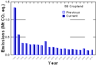
Fig. 7.11 Current and previously reported assessment of emissions for category 5B Cropland.

7.4.6 Source-specific planned improvements

Similarly as for other categories, additional efforts will be exerted to further consolidate the current estimates for Cropland. Specific attention will be paid to a likely overall formalization and enhancement of the QA/QC procedures. Also, a more detailed stratification of Cropland area to allow a more specific application of appropriate factors used in emission estimation will be explored as also suggested by the latest in-country review.

7.5 Grassland (5C)

7.5.1 Source category description

Through its spatial share of close to 14 % in 2010, the category of Grassland ranks third among land-use categories in the Czech Republic. Its area has been growing since 1990, specifically in early 1990s (Fig. 7.4). Grassland as defined in this inventory corresponds to the grassland real estate category, one of the six such categories of agricultural land in the database of “Aggregate areas of cadastral land categories” (AACLC), collected and administered by COSMC. This land is mostly used as pastures for cattle and meadows for growing feed. Additionally, the fraction of permanently unstocked cadastral Forest Land is also included under Grassland. This is because it predominantly has the attributes of Grassland (such as land under power transmission lines).

The importance of Grassland will probably increase in this country, both for its production role and for preserving biodiversity in the landscape. According to the national agricultural programs, the representation of Grassland should further increase to about 18 % of the area of the country. The dominant share should be converted from Cropland, the share of which is still considered excessive. After implementation of subsidies in the 1990s, the area of Grassland has increased by about 17 % (in 2010) since 1990.

Fig. 7.12 Grassland in the Czech Republic – distribution calculated as a spatial share of the category within individual cadastral units (as of 2010).

7.5.2 Methodological aspects

The emission inventory of 5C Grassland concerns sub-categories 5C1 Grassland remaining Grassland and 5C2 Land converted to Grassland. Similarly to 5B Cropland, the emission inventory of 5C Grassland considers changes in living biomass and soil. In addition, the effect of application of agricultural limestone is quantified for this category.

7.5.2.1 Grassland remaining Grassland

For category 5C1 Grassland remaining Grassland, the assumption of no change in carbon stock held in living biomass was employed, in accordance with the Tier 1 approach of IPCC (2003). This is a safe assumption for the conditions in this country and any application of higher tier approaches would not be justified with respect to data requirements and the expected insignificant carbon stock changes.

The emissions estimates from changes in soil carbon stock were estimated for category 5C1. These changes are due to an effect of different management regimes and the changing proportion of the concerned subcategories of 5C1. The changes also concern permanently unstocked cadastral Forest Land, which has the attributes of Grassland and is treated accordingly in the emission estimates (see Section 7.3.1). Other land belonging to the category of Grassland is considered as typically managed grassland. The reference soil carbon stock for this category is estimated as area-weighted mean for all the individual cadastral units. The analogous mean carbon content for the category of unmanaged grassland is determined using the corresponding factors (Table 5.5; IPCC 2006). These included the stock change factor for land use (F_LU; 1.0), stock change factor for the management regime (F_MG; 0.95) and stock change factor for input of organic matter (F_I; 1.0). The estimated area-weighted average soil carbon stock for classically managed grassland was equal to 69 t C/ha, while that for unmanaged grassland was 65.5 t/ha. This is estimated for the whole reporting period and the soil carbon stock change was derived from the difference between the consecutive years. The changes in soil carbon stock associated with the annually changing proportion of land areas of cropland sub-categories result in emissions/removals. These are calculated after redistribution of the estimated carbon stock change over a 20-year rolling period.

Other explicitly quantified effect on soil carbon that results in CO₂ emissions is that of limestone application. This was quantified as described in Section 7.3.2.1 for 5B Cropland. The applicable amount of limestone was set at 5 % of the reported limestone use on agricultural lands, based on expert judgment (V. Klement, Central Institute for Supervising and Testing in Agriculture – personal communication, 2005).

Non-CO₂ gases on category 5C1 Grassland remaining Grassland do not concern the LULUCF sector in the Czech Republic.

7.5.2.2 Land converted to Grassland

For category 5C2 Land converted to Grassland, the estimation concerns carbon stock changes in living biomass and soils.

For living biomass, the calculation used Eq. 3.4.13 (IPCC 2003) with the assumed carbon content before the conversion of 5B Cropland set at 5 t C/ha (Table 3.4.8; IPCC 2003) and that of Forest Land calculated from the mean growing stock volumes as described in Section 7.3.2.2 above. The biomass carbon content immediately after the conversion was assumed to equal zero and carbon stock from one-year growth of grassland vegetation following the conversion was assumed to be 6.8 t C/ha (Table 3.4.9; IPCC 2003).

For dead organic matter, emissions are reported due to changes in deadwood that concern the category 5C21 Forest Land converted to Grassland. Apart from the actual areas concerned, the emission estimation is identical as described in Section 7.4.2.2 above.

The estimation of carbon stock change in soils for category 5C2 Land converted to Grassland in the Czech Republic concerns the changes in mineral soils. The soil carbon stock changes following the conversion from 5A Forest Land and 5B Cropland were quantified by the country-specific Tier 2/Tier 3 approach described in detail in Section 7.2.2.2 above.

7.5.3 Uncertainties and time series consistency

Similarly as for other land-use categories, the methods used in this inventory for Grassland were consistently employed across the whole reporting period from the base year of 1990 to 2010. The uncertainty estimation was guided by the Tier 1 methods outlined in GPG for LULUCF (IPCC 2003) and described in Section 7.3.3. The uncertainty estimation utilized primarily the default uncertainty values as recommended by IPCC (2003, 2006). As reported above in chapter 7.3.3, uncertainty estimation was revised for this submission, which applies also to this land use category. The following uncertainty values were used: converted land use areas 3 %, average growing stock volume in forests prior conversion 8 %, average biomass stock in cropland and grassland prior conversion 75 %, biomass carbon stock after land-use conversion 75 %, average amount of standing deadwood 27 %, average amount of lying deadwood 20 %, average above-ground to below-ground biomass ratio R (root-shoot-ratio) 68 %, stock change factor for land use 50 %, stock change factor for management regime 5 %, amount of lime 10 %, emission factor for liming 5 % and reference biomass carbon stock prior to and after land-use conversion 75 %. The uncertainty applicable to BCEF was 22 %, which was derived from the work of Lehtonen et al. (2007).

For 2010, the total estimated uncertainty for category 5C1 Grassland remaining Grassland reached 9.5 %. The corresponding uncertainty for category 5C2 Land converted to Grassland reached 18.0 %. The overall combined uncertainty for category 5C Grassland also reached 18.1 %.

7.5.4 QA/QC and verification

The emission estimates are based on the activity data taken from the official national sources and follow the recommendations of GPG for LULUCF. Data sources are verifiable and updated annually. All the input information and calculations are archived by the expert team and the coordinator of NIR. Hence, all the background data and calculations are verifiable. Other QA/QC elements were adopted in the same manner as described in Section 7.3.4 above, following the application of the QA/QC plan applicable for the LULUCF sector.

7.5.5 Recalculations

No recalculation has been performed in the category of Grassland since the last submission. Therefore, the current and previous estimates are identical for the jointly reported years (Fig. 7.13).

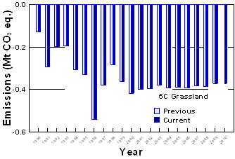
Fig. 7.13 Current and previously reported assessment of emissions for category 5C Grassland. The values are negative, hence representing net removals of green-house gases.

7.5.6 Source-specific planned improvements

Further efforts to consolidate the emission estimates are expected for the category of Grassland. Specific attention will be paid to a likely overall formalization and enhancement of the QA/QC procedures. Also, a more detailed stratification of Grassland area to allow a more specific application of factors used in emission estimation will be explored.

7.6 Wetlands (5D)

7.6.1 Source category description

Category 5D Wetlands as classified in this emission inventory includes riverbeds, and water reservoirs such as lakes and ponds, wetlands and swamps. These areas correspond to the real estate category of water area of the “Aggregate areas of cadastral land categories” (AACLC), collected and administered by COSMC. It should be noted that there are about 11 wetlands identified as Ramsar [20] sites in this country. However, these areas are commonly located in several IPCC land-use categories and are not directly comparable with the actual content of the 5D emission category.

The area of 5D Wetlands currently covers 2.1 % of the total territory. It has been growing steadily since 1990 (Fig. 7.4) with even a stronger trend since 1970. It can be expected that this trend would continue and that the area of Wetlands would increase further. This is mainly due to programs aimed at increasing the water retention capacity of the landscape[21].

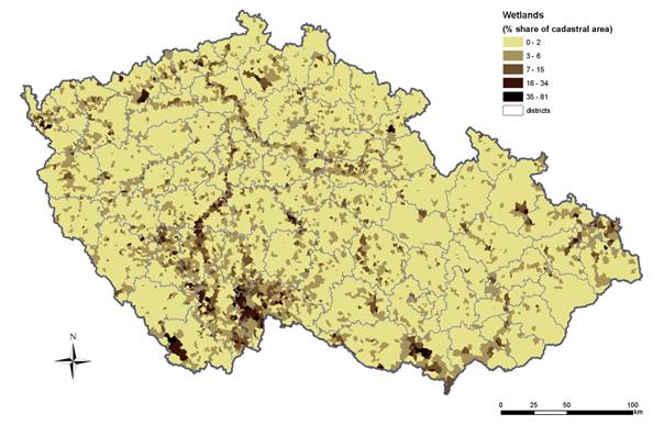
Fig. 7.14 Wetlands – distribution calculated as a spatial share of the category within individual cadastral units (as of 2010).

7.6.2 Methodological aspects

The emission inventory of sub-category 5D1 Wetlands remaining Wetlands can address the areas in which the water table is artificially changed, which correspond to peat-land draining or lands affected by water bodies regulated through human activities (flooded land). Both categories are insignificant under the conditions in this country. Hence, the emissions for 5D1 Wetlands remaining Wetlands were not explicitly estimated and they can safely be considered negligible.

Sub-category 5D2 Land converted to Wetlands encompass conversion from 5A Forest Land, 5B Cropland and 5C Grassland. This is a very minor land-use change identified in this country, which corresponds to the category of land converted to flooded land. The emissions associated with this type of land-use change are derived from the carbon stock changes in living biomass and in the case of conversion from Forest land, also deadwood. The emissions were generally estimated using the Tier 1 approach and Eq. 3.5.6 of GPG for LULUCF, which simply relates the biomass stock before and after the conversion. The corresponding default values were employed: the biomass stock after conversion equaled zero, while the mean biomass stock prior to the conversion in the 5A Forest Land, 5B Cropland and 5C Grassland categories was estimated and/or assumed identically as described above in Sections 7.3.2.2 and 7.4.2.2. The latter section also describes the estimation of emissions related to deadwood component, which was applied identically in this land use category.

7.6.3 Uncertainties and time series consistency

The methods used in this inventory for Wetlands were consistently employed across the whole reporting period from the base year of 1990 to 2010. Similarly as for the other land-use categories, the uncertainty estimation was guided by the Tier 1 methods outlined in GPG for LULUCF (IPCC 2003) and described in Section 7.3.3. It utilized primarily the default uncertainty values as recommended by IPCC (2003, 2006). As reported above in chapter 7.3.3, uncertainty estimation was revised for this submission, which applies also to this land use category. The following uncertainty values were used: converted land use areas 3 %, average growing stock volume in forests prior conversion 8 %, average biomass stock in cropland and grassland prior conversion 75 %, biomass carbon stock after land-use conversion 75 %, average amount of standing deadwood 27 %, average amount of lying deadwood 20 %, carbon fraction of dry woody matter 7 %, and average above-ground to below-ground biomass ratio R (root-shoot-ratio) 68 %. The uncertainty applicable to BCEF was 22 %, which was derived from the work of Lehtonen et al. (2007).

Since the emission estimate concerns only category 5D2 Land converted to Wetlands, the uncertainty is estimated for this category. For 2010, the estimated uncertainty for category 5D2 was 71 %.

7.6.4 QA/QC and verification

7.6.5 Recalculations

No recalculation has been performed in the category of Wetlands since the last submission. Therefore, the current and previous estimates are identical for the jointly reported years (Fig. 7.15).

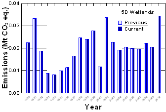
Fig. 7.15 Current and previously reported assessment of emissions for the category 5D Wetlands.

7.6.6 Source-specific planned improvements

For the category of 5D Wetlands, attention will be paid to a further consolidation of the uncertainty assessment and to overall formalization and enhancement of the QA/QC procedures.

7.7 Settlements (5E)

Fig. 7.16 Settlements – distribution calculated as a spatial share of the category within individual cadastral units (as of 2010).

7.7.1 Source category description

Category 5E Settlements is defined by IPCC (2003) as all developed land, including transportation infrastructure and human settlements. For this emission inventory, the area definition under category 5E Settlements was revised to better match the IPCC (2003) default definition. The category currently includes two categories of the database “Aggregate areas of cadastral land categories” (AACLC), collected and administered by COSMC, namely “Built-up areas and courtyards” and “Other lands”. Of the latter AACLC category, all types of land-use were included with the exception of “unproductive land”, which corresponds to category 5F Other Land. Hence, the Settlements category also includes all land used for infrastructure, as well as that of industrial zones and city parks, previously included in category 5F Other Land.

The category of Settlements as defined above currently represents about 8.6 % of the area of the country. The area of this category has increased since 1990 and especially during the most recent years (Fig. 7.4).

7.7.2 Methodological aspects

The emission inventory for this category concerns primarily 5E2 Land converted to Settlements. As for category 5E1 Settlements remaining Settlements, emissions of CO₂ were considered insignificant as no change in biomass, dead organic matter and soil carbon pools is assumed (Tier 1, IPCC 2006). Emissions quantified in this inventory concern the category 5E2 Forest Land converted to Settlements. The emissions result mainly from the biomass carbon stock change, which was quantified using Eq. 3.6.1 (IPCC 2003). The carbon stock prior conversion was estimated as described in Section 7.3.2.2. All biomass is assumed to be lost during the conversion, according to the Tier 1 assumption of GPG for LULUCF. Additional contribution to emissions is from deadwood component. It was estimated identically as described in Section 7.4.2.2 above, using the actual areas of the land use change concerned.

7.7.3 Uncertainties and time series consistency

The methods used in this inventory for 5E Settlements were consistently employed across the whole reporting period from the base year of 1990 to 2010. The uncertainty estimation was guided by the Tier 1 methods outlined in GPG for LULUCF (IPCC 2003) and described in Section 7.3.3. It utilized primarily the default uncertainty values as recommended by IPCC (2003, 2006). As reported above, uncertainty estimation was revised for this submission, which applies also to this land use category. The following uncertainty values were used: carbon fraction in dry matter 7 %, land use areas 3 %, reference biomass carbon stock prior and after land-use conversion 75 %, average growing stock volume in forests 8 %, average amount of standing deadwood 27 %, average amount of lying deadwood 20 %, and average above-ground to below-ground biomass ratio R (root-shoot-ratio) 68 %. The uncertainty applicable to BCEF was 22 %, which was derived from the work of Lehtonen et al. (2007).

The emission estimate concerns only category 5E2 Land converted to Settlements; therefore, the uncertainty is estimated only for this category. For 2010, the estimated uncertainty for the category 5E2 was 102 %.

7.7.4 QA/QC and verification

7.7.5 Recalculations

Similarly as for the other categories, no recalculation has been performed in the category of Settlements since the last submission. Therefore, the current and previous estimates are identical for the jointly reported years (Fig. 7.17).

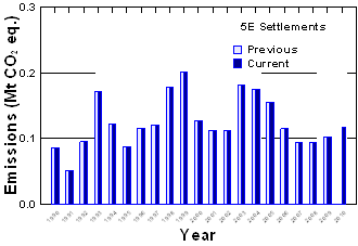
Fig. 7.17 Current and previously reported assessment of emissions for the category 5E Settlements.

7.7.6 Source-specific planned improvements

Further efforts to consolidate the emission estimates are expected for the category of Settlements. This will include an assessment of how the data from the recently conducted statistical landscape inventory CzechTerra (Černý 2009) could be utilized. Attention will also be paid to further improvement of the uncertainty assessment and overall formalization and enhancement of the QA/QC procedures.

7.8 Other Land (5F)

7.8.1 Source category description

Since NIR 2008 submission, the category 5F Other Land represents unmanaged (unmanageable) land areas, matching the IPCC (2003) default definition. These areas were assessed from the database of “Aggregate areas of cadastral land categories” (AACLC), collected and administered by COSMC. It is a part the AACLC category “other lands” with the specific land use category “unproductive land”, assessed from the 2006 land census of COSMC. This category represents 1.0 % of the territory of the country and it is considered to be constant, not involving any land-use conversions.

7.8.2 Methodological aspects

Change in carbon stocks and non-CO₂ emissions are not considered for 5F1 Other Land remaining Other Land (IPCC 2003). Since no land-use conversion involving “other land” is assumed by this inventory, no emissions were considered in the entire category 5F Other Land.

7.8.3 Uncertainties and time series consistency

The uncertainty estimates are not reported here. Time series consistency is ensured as the inventory approaches and/or assumptions are applied identically across the whole reporting period from the base year 1990 to 2010.

7.8.4 QA/QC and verification

The activity data are based on land-use information from the national sources and the estimation approaches follow the recommendations of GPG for LULUCF.

The QA/QC elements were adopted in the same manner as described in Section 7.3.4 above, limited to those relevant for this specific land-use category.

7.8.5 Recalculations

No recalculations concern category 5F Other Land.

7.8.6 Source-specific planned improvements

There are no short-term plans concerning this category.

7.9 Other (5G)

7.9.1 Source category description

Since this submission, the category 5G Other is reported . Unlike other land use categories, 5G Other has no area representation and therefore it is not reported in land use matrices (Tab. 7.3). It was introduced to facilitate reporting of emissions from lime application on Forest land. This is due to the current technical restrictions of the CRF Reporter software, which does not permit adding emissions from lime application under the category of 5A Forest Land where these emissions should actually be attributed to.

7.9.2 Methodological aspects

For the emissions from lime application, the methodology described in Section 3.3.1.2.1 of GPG for LULUCF (IPCC 2003) was used. The activity data in terms of forest area and amount of limestone applied were taken from the national reports on Czech forestry (Green report, MA 2011). In 2010, the amount of lime applied to forest soils equaled 5.12 kt and concerned an area of 1 721 ha.

7.9.3 Uncertainties and time series consistency

The uncertainty estimates are not specifically reported here. Time series consistency is ensured as the inventory approaches and/or assumptions are applied identically across the whole reporting period from the base year 1990 to 2010.

7.9.4 QA/QC and verification

The activity data are based on land-use information from the national sources and the estimation approaches follow the recommendations of GPG for LULUCF.

The QA/QC elements were adopted in the same manner as described in Section 7.3.4 above, limited to those relevant for this specific emission category.

7.9.5 Recalculations

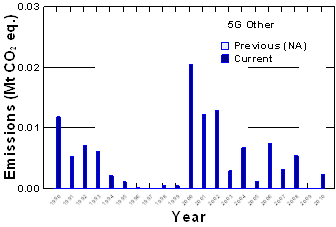
Fig. 7.18 Currently reported assessment of emissions for the category 5G Other, represented solely by emissions from lime application on Forest land. Not applicable (NA) for the previous submission.

Since the category 5G Other is used and reported for the first time, no recalculations are applicable for this category (Fig. 7.18).

7.9.6 Source-specific planned improvements

The UNFCCC Secretariat will be further consulted to allow reporting of the emissions from lime application on forest land under the category 5A Forest Land, where it logically belongs. Once this will be made possible in the CRF Reporter, the category 5G Other will not be used for this purposes.

7.10 Acknowledgement

The authors would like to thank Vladimír Henžlík, formerly at the Forest Management Institute in Brandýs n. Labem, for some of the activity data and his expert advice. Thanks are also due to Jan Hána, Patrik Pacourek and Miroslav Zeman, Forest Management Institute in Brandýs n. Labem, for compiling the required increment data concerning forests. Some of the analyses required for this inventory were performed within the project CzechCarbo (VaV/640/18/03), while some of the critical data were obtained from the project CzechTerra (SP/2d1/93/07), both funded by the Czech Ministry of the Environment.

8 Waste (CRF sector 6)

8.1 Overview

The waste sector consists of several categories. The main source category of this sector is 6A Methane emissions from solid waste disposal sites. In 2010, this category emitted 124 Gg of methane (2612 Gg of CO₂ ekv). The second source category is 6B emissions from waste-water, which is calculated as the sum of four subcategories – emissions of methane from industrial waste-water treatment, domestic waste-water treatment, on-site treatment and emissions of nitrous oxide from waste-water. These subcategories summed up in 2009 emitted 24.2 Gg of methane and 0.66 Gg of N₂O. The last source category in this sector is incineration of wastes, which was recalculated this year and split between two sectors. Waste used as a fuel for energy purposes was calculated and reported in category 1AA1A other fuels. Industrial and hazardous waste remained in category 6 C and produced a total of 183 Gg of fossil CO_2ekv.This inventory year sector 6 produced 3515 Gg of CO_2ekv in total.

Tab. 8‑1 Overview of significant categories in this sector (2010)

Category	Character of category	Gas	% of total GHG*
6A Solid Waste Disposal on Land	KC (LA, TA, LA, TA)	CH₄	2.0
6B Waste Water Handling	non-KC	CH₄	0.4
6C Waste Incineration (without MSW)	non-KC	CO₂	0.1
6B Waste Water Handling	non-KC	N₂O	0.1

* assessed without considering LULUCF

KC: key category,LA, LA*: identified by level assessment with and without considering LULUCF, respectively

TA, TA*: identified by trend assessment with and without considering LULUCF, respectively

Right from the start, CHMI co-operated in compilation of the emission inventory for this sector with professional workplaces, in particular with the Institute for Environmental Science of the Faculty of Sciences at Charles University in Prague (PřFUK) (Havránek, 2001), the University of Chemical Technology (VŠCHT) (Zábranská, 2004) and the Institute for Research and Use of Fuels in Prague Běchovice (ÚVVP) (Straka, 2001). In the framework of this cooperation, all the emission inventories in this category were recalculated for the entire time series from the reference year of 1990 to the present. At the present time, this sector is managed by the Charles University Environmental Center (CUEC).

8.2 Solid Waste Disposal on Land (6A)

8.2.1 Source category description

Treatment and disposal of municipal, industrial and other solid waste produces significant amounts of methane (CH₄). Decomposition of organic material derived from biomass sources (e.g., crops, wood) is the primary source of CO₂ released from waste. These CO₂ emissions are not included in the national totals, because the carbon is of biogenic origin and net emissions are accounted for under land use change and forestry.

This category produces emissions of other micropollutants, such as non-methane volatile organic compounds (NMVOCs), as well as smaller amounts of nitrous oxide (N₂O), nitrogen oxides (NO_x) and carbon monoxide (CO). Only CH₄ is addressed in this report.

Category was recalculated for this year. Based on suggestions in the in-country review, we gathered country-specific waste composition data. Using the default carbon content suggested in the IPCC guidelines, we derived the country-specific DOC for particular waste streams.

8.2.2 Methodological issues

Waste disposal to SWDS

Key activity data for methane quantification from 6.A consists in the amount of waste disposed in landfills. Annual disposal is shown Tab. 8‑2 MSW disposal in SWDS in the Czech Republic [Gg], 1990-2010. Data for annual disposal are from mixed sources because correct application of the FOD model requires data from 1950 to the present day. These data are not available in the country and therefore assumptions about the past must have been used. These assumptions are described in the working paper published in this issue (Havránek, 2007) but the method can be simply described as intrapolation and extrapolation between points in time; we correlated waste production with social product (predecesor of current GDP) as a test method. The higher of the two estimates was used in the quantification.

Tab. 8‑2 MSW disposal in SWDS in the Czech Republic [Gg], 1990-2010

Year	MSW in SWDS	Year	MSW in SWDS	Year	MSW in SWDS
1990	2371	1997	2739	2004	3000
1991	2388	1998	2804	2005	3070
1992	2484	1999	2632	2006	3221
1993	2543	2000	2803	2007	3314
1994	2561	2001	2826	2008	3424
1995	2621	2002	2920	2009	3406
1996	2683	2003	2952	2010	3185

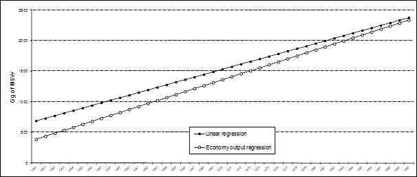
Fig. 8‑1MSW disposal in SWDS in the Czech Republic, 1950-1990

The method used for estimation of methane emissions from this source category is the Tier 2 FOD approach (first-order decay model). The first-order decay (FOD) model assumes gradual decomposition of waste disposed in landfills. We calculated GHG emissions from the IPCC Spreadsheet for Estimating Methane Emissions from Solid Waste Disposal Sites, which is part of the new methodology guidelines (IPCC, 2007) referred further to as (IPCC model, 2006).

Waste composition, k-rate and DOC

Waste composition is crucial for emission estimations. We made several attempts to obtain country-specific data about waste composition. Light-greyed data (1990-1995) are based on the IPCC default values for Eastern Europe, Dark-greyed data (1996-2000 and 2002-2004) are based on intrapolation between data points. Data in the white rows (2001 and 2005-2010) are based on waste surveys performed in R&D projects dealing with waste composition.

The table also contains the methane generation rate (k-rate) employed. This rate is closely related to the compostion of a particular substance and the available moisture. We used IPCC default k-rates for a wet temperate climate (as the average temperature of the Czech Republic is about 7 °C and the annual precipitation is higher than the potential evapotranspiration). The average DOC for particular waste streams is also based on the IPCC default values for particular categories of waste. The average DOC for a particular year is in the last column of the table.

Tab. 8‑3 MSW composition for the Czech Republic used in the quantification (fractions of total, 1990-2010)

	Paper	Food	Textil	Wood and straw	DOC
k-rate	0.06	0.185	0.06	0.03
DOC	0.4	0.15	0.24	0.43
	Share of particular waste streams
1990	0.22	0.30	0.05	0.08	0.176
1991	0.22	0.30	0.05	0.08	0.176
1992	0.22	0.30	0.05	0.08	0.176
1993	0.22	0.30	0.05	0.08	0.176
1994	0.22	0.30	0.05	0.08	0.176
1995	0.22	0.30	0.05	0.08	0.176
1996	0.22	0.29	0.05	0.08	0.179
1997	0.23	0.28	0.06	0.08	0.181
1998	0.24	0.27	0.06	0.08	0.184
1999	0.25	0.26	0.07	0.08	0.187
2000	0.26	0.25	0.07	0.08	0.191
2001	0.27	0.23	0.08	0.08	0.195
2002	0.24	0.25	0.08	0.09	0.194
2003	0.22	0.27	0.07	0.11	0.193
2004	0.19	0.30	0.07	0.13	0.192
2005	0.16	0.32	0.07	0.14	0.191
2006	0.16	0.32	0.07	0.14	0.187
2007	0.17	0.32	0.08	0.13	0.193
2008	0.16	0.32	0.07	0.14	0.188
2009	0.16	0.35	0.08	0.13	0.193
2010	0.16	0.35	0.08	0.13	0.193

Methane correction factor

The methane correction factor (MCF) is a value expressing overall management of the landfills in the country. Better-managed and deeper landfills have larger MCF values. Shallow SWDS ensure that far more oxygen penetrates into the body of the landfill to aerobically decompose DOC. The suggested IPCC values are given in Tab. 8‑4 Methane correction values (IPCC, 1996)

Tab. 8‑4 Methane correction values (IPCC, 1996)

	MCF
Unmanaged, shallow	0.4
Unmanaged, deep	0.8
Managed	1.0
Managed, semi-aerobic	0.5
Uncategorised	0.6

Tab. 8‑5 MCF values employed, 1950-2010

	MCF
1950 – 1959	0.6
1960 – 1969	0.6
1970 – 1979	0.8
1980 – 1989	0.9
1990 – 2010	1.0

Oxidation factor

As methane moves from the anaerobic zone to the aerobic and semi-aerobic zones close to the landfill surface, part of it becomes oxidized to CO₂. There is no conclusive agreement in the scientific community on how intensive the oxidation of methane is. Oxidation is indeed site-specific due to the effects of local conditions (including fissures and cracks, compacting, landfill cover etc.). No representative measurement or estimations of the oxidation factor are available for the Czech Republic. Some studies are quoted in Straka, 2001, which mentions a non-zero oxidation factor, but these figures seem to be site-specific (and really high) and therefore cannot be used as representative for the whole country. However, the methodology (IPCC, 2000) suggests that an oxidation factor higher than 0.1 should not be used if no site measurements are available (a larger value adds uncertainty). The author used the recommended oxidation factor of 0.1 in the report.

Delay time

When waste is disposed in SWDS, decomposition (and methanogenesion) do not start immediately. The assumption employed in the IPCC model is that the reaction starts on the first of January in the year after deposition, which is equivalent to an average delay time of six months before decay to methane commences. It is good practice to assume an average delay of two to six months. If a value greater than six months is chosen, evidence to support this must be provided. The Czech Republic has no representative country-specific value for delay time, so the author used a default value of 6 months.

Fraction of methane

This parameter indicates the share (mass) of methane in the total amount of Landfill Gas (LFG). In previous calculations of methane emissions from SWDS (NIR, 2004), a value 0.61 was used. This figure was based on measurement of a limited number of sites (Straka, 2001). This value is higher than the range of 0.5-0.6 suggested by IPCC. In this work, we revised these values based on new evidence (MIT, 2005). MIT receives annual reports from landfills capturing their LFG; SWDS report the net calorific value of their captured LFG. We used this value for comparison with the gross calorific value of pure methane, yielding a value of approx. 0.55, which was used in the quantification.

Recovered methane

On SWDS in the country, methane is sometimes collected by an LFG collection system and incinerated for energy purposes. Based on IPCC guidelines, this methane is converted to CO₂ and, having biogenic origin, it is not considered to constitute an emission of GHG. Recovered methane (R) is substituted in the equation in Appendix 1. There is no default value for R, so we used country estimates based on various sources. The Ministry of Industry and Trade conducts an annual survey of all SWDS. All the energy data about LFG is collected. An attempt is made to update old estimates as much as possible. Since the start of the survey in 2005, it has been possible to provide estimates for time series from 2003 to 2010. The estimates in Straka, 2001 were used for the 1990-1996 period. Linear intrapolation of recovered methane was used for the period between 2003 and 1996.

CH₄ recovery column. Because of changes in the activity data on methane recovery provided by MIT, the time series since 1996 has been recalculated.

Total emissions of methane are based on the equation from the IPCC CH₄ model. Detailed time series from 1950 with breakdown into individual waste components are given in the paper by Havranek 2007, together with the other model outputs gives the trends in emissions of methane from SWDS following recalculation.

Tab. 8‑6 Emissions of methane from SWDS [Gg], Czech Republic, 1990-2010

	CH₄ generation	CH₄ recovery	CH₄ oxidized	CH₄ emission
1990	91	3.3	9.1	79.2
1991	95	3.3	9.5	82.8
1992	99	3.5	9.9	86.0
1993	103	3.5	10.3	89.5
1994	107	3.5	10.7	93.0
1995	110	3.5	11.0	96.2
1996	114	6.0	11.4	97.1
1997	118	6.6	11.8	99.9
1998	121	7.1	12.1	102.6
1999	125	7.7	12.5	105.5
2000	127	8.2	12.7	107.3
2001	131	8.8	13.1	109.8
2002	134	9.3	13.4	112.3
2003	138	9.9	13.8	115.1
2004	142	15.6	14.2	113.4
2005	145	18.0	14.5	114.7
2006	149	20.6	14.9	116.0
2007	154	25.9	15.4	114.8
2008	158	24.6	15.8	120.4
2009	163	24.5	16.3	124.5
2010	168	24.7	16.8	129.0

8.2.3 Uncertainties and time-series consistency

This sector was extensively recalculated this year. We changed waste composition to be consistent with the country estimates and we have changed recovered methane estimates to be consistent with the latest data collection work on LFG. Havranek, 2007 contains a sensitivity analysis for several key factors and assumption used in the previous recalculation when we moved from Tier 1 to Tier 2. Overall quantification of the uncertainity for this category is still incomplete. This is considered a high priority and will be conducted in the following years as soon as budget constraints permit. This category entails the difficulty that the uncertainty does not permeate through the whole waste management period of 1950-2010 and cannot be quantified by simple analysis.

8.2.4 QA/QC and verification

Activity data from national agencies and ministries are the subjects of internal QA/QC mechanisms. The recalculation that is fully described in Havranek, 2007 was approved by the Expert Review Team in 2007.

8.2.5 Recalculations

Several changes in this sector qualify as recalculation. The first small change is in the amount of MSW that is disposed in SWDS. This change is due to improved data available for this activity and it is a minor change (less than 1%). The second major change is the use of country-specific values for waste composition. Due to the higher-than-default values mainly in the food category, this led to changes in the total DOC in landfilled waste and increased methane emissions significantly. The third change was in the estimate of recovered methane . Here, we used actualized data from the statistical survey

8.2.6 Sector specific improvements

We have improved this sub-category this year by using country specific values for the waste. In near future we do not plan any significant methodological improvement. We plan to conduct uncertainity analysis of the newly recalculated results in 2013 submission. We of course will include improved data in this category should they be available but not as a planned improvement but rather as regular maintenance of the quality of the chapter.

8.3 Waste-water Handling (6B)

8.3.1 Source category description

This category has CRF code 6B and consists of four separately calculated sub-categories – emissions of methane from 6B1 Industrial Waste-water, 6B2 Domestic and Commercial Waste-water and 6B3 Other (Treatment on site) and emissions of nitrous oxide from 6B2 Domestic and Commercial Waste-water.

8.3.2 Methodological issues

The basic factor for determining methane emissions from waste-water handling is the content of organic pollution in the water. The content of organic pollution in municipal waste-water and sludge is given as BOD₅ (the biochemical oxygen demand). BOD is a group method of determination of organic substances and expresses the amount of oxygen consumed in the biochemical oxidation, and is thus a measure of biologically degradable substances. In contrast, COD (chemical oxygen demand) is the amount of oxygen required for chemical oxidation and includes both biologically degradable and biologically non-degradable substances. COD is used according to the Revised 1996 IPCC Guidelines, 1997 for calculation of methane emissions from industrial waste-water and is always larger than BOD.

The current IPCC methodology employs BOD for evaluation of municipal waste-waters and sludge and COD for industrial waste-waters. The new method is also extended to include determination of emissions from sludge that are primarily the products of various methods of treatment of waste-waters and, under anaerobic conditions, may contribute to methane production and methane emissions. The amount of nitrous oxide emitted from waste-waters is a function of protein consumption in the population rather than BOD or COD.

8.3.2.1 Industrial waste-water (6B1)

The main activity data for estimation of methane emissions from this subcategory is determination of the amount of degradable pollution in industrial waste-water. In this inventory we use specific production of pollution - the amount of pollution per production unit - kg COD / kg product and then we multiply it by the production, or the value obtained from the overall amounts of industrial waste-water and from a qualified estimate of their concentrations (in kg COD/m³). We use the procedure from the IPCC methodology (Revised 1996 IPCC Guidelines, 1997; Good Practice Guidance, 2000). The necessary activity data were taken from the material of CZSO (Czech Statistical Office - Statistical Yearbook) and the other parameters required for the calculation were taken from the IPCC Good Practice (Good Practice Guidance, 2000). On the basis of information on the total amount of industrial waste-water equal to 159 mil.m³ (actually only 157 mil.m³ were treated) (Source CENIA, Environmental Statistical Yearbook) we are able to correct our overestimation of possible waste-water generation of industry (40 mil.m³), which was assigned an average concentration of 3 kg COD/m³. In previous years this factor was positive; in 2008, for the first time, this correction factor started to be negative. In addition, in accordance with (Revised 1996 IPCC Guidelines, 1997), it was estimated that the amount of sludge equals 10% of the total pollution in industrial water (25% was assumed in the Meat & Poultry, Paper and Pulp and in Vegetables, Fruits & Juices category). These estimates are based on Dohanyos and Zábranská, 2000; Zábranská, 2004, see Tab. 8‑7 Estimation of COD generated by individual sub-categories 2010.

Tab. 8‑7 Estimation of COD generated by individual sub-categories 2010

	Production [kt/year]	COD/m³ [kg /m³]	Waste-water/t [m³/t]	Share of sludge [%]	COD of sludge [t]	COD of waste-water [t]
Alcohol Refining	16	11.0	24.00	0.10	423	3 804
Dairy Products	1 118	2.7	7.00	0.10	2 113	19 017
Malt & Beer	3 281	2.9	6.30	0.10	5 994	53 950
Meat & Poultry	504	4.1	13.00	0.25	6 716	20 147
Organic Chemicals	183	3.0	67.00	0.10	3 690	33 213
Pet. ref./Petrochemicals^{^[22]}	0	1.0	0.60	0.10	0	0
Plastics and Resins	600	3.7	0.60	0.10	133	1 199
Pulp & Paper	830	9.0	162.00	0.25	302 717	908 152
Soap and Detergents	29	0.9	3.00	0.10	7	67
Starch production	83	10.0	9.00	0.10	748	6 733
Sugar Refining	421	3.2	9.00	0.10	1 213	10 920
Textiles(natural)	36	0.9	172.00	0.10	556	5 002
Vegetable Oils	122	0.9	3.10	0.10	32	289
Vegetables, Fruits & Juices	120	5.0	20.00	0.25	2 985	8 954
Wine & Vinegar	59	1.5	23.00	0.10	204	1 839
*Unidentified waste-water*	- 38 865	3.0	1.00	0.10	-11 659	-104 935
Total					315 873	968 352

Tab. 8‑8 Parameters for CH₄ emissions calculation from industrial waste-water 1990-2010

	MCF	1990	1993	1996	1999	2002	2005	2008	2009	2010
Non-treated	0.05	29 %	18 %	13 %	5 %	7 %	3 %	1 %	2%	1%
Aerobic treatment of water	0.06	67 %	73 %	70 %	70 %	65 %	68 %	69 %	69%	70%
Anaerobic treatment of water	0.70	4 %	8 %	17 %	25 %	28 %	29 %	30 %	30%	29%
Aerobic treatment of sludge	0.10	40 %	40 %	40 %	40 %	30 %	27 %	27 %	27%	27%
Anaerobic treatment of sludge	0.30	60 %	60 %	60 %	60 %	70 %	73 %	73 %	73%	73%

In accord with (Good Practice Guidance, 2000), the maximum theoretical methane production B₀ was considered to equal 0.25 kg CH₄/kg COD. This value is in accordance with the national factors presented in Dohanyos and Zábranská, 2000.

The calculation of the emission factor for waste-water is based on a qualified estimate of the ratio of the use of individual technologies during the entire recalculated time series. In the future, this ratio will shift towards anaerobic treatment of waste-water and sludge because of the energy advantages of this means of treating waste-water. Tab. 8‑7 Estimation of COD generated by individual sub-categories 2010 describes this trend. The conversion factor for anaerobic treatment is 0.06 and, for aerobic treatment, 0.7.

In contrast to a quite stable ratio for waste-water treatment technologies (6.B.2), ratio used for sludge keeps shifting in favor of anaerobic treatment. This is mostly due its economic efficiency. The calculation of the emission factor for sludge was based on the assumption that 27% is treated anaerobically with a conversion factor of 0.3 and the remaining 73 % by other, especially aerobic methods with a conversion factor of 0.1. Similarly as in 6.B.2, it is assumed that all the methane from anaerobic processes is burned (mostly usefully in cogeneration units, as flaring is being phased out and cogeneration technology seems to be economically effective); however, in contrast to municipal water, methane from anaerobic sludge and waste-water is included. This assumption is based on national standards and regulations presented in the subchapter below (Zábranská, 2004). For calculation of methane emissions, it is sufficient to consider only aerobic processes (where the methane is not oxidized to biological CO₂). Experts at the University of Chemical Technology recommended the conversion factors and other parameters given in this part, see (Dohanyos and Zábranská, 2000; Zábranská, 2004).

Tab. 8‑9 Emissions of CH₄ (Gg) from 6B1, 1990-2010, Czech Republic

	1990	2000	2001	2002	2003	2004	2005	2006	2007	2008	2009	2010
CH₄ production	49.8	63.5	66.4	77.4	75.4	77.4	76.9	80.6	80.9	78.0	76.0	79.8
Oxidized CH₄	25.3	50.3	55.5	64.5	63.0	65.0	64.7	67.9	68.1	65.9	64.2	67.5
Total CH₄ emissions	24.5	13.3	10.9	12.9	12.3	12.2	12.1	12.7	12.3	12.1	11.8	12.3

8.3.2.2 Municipal and commercial waste-water treatment (6B2) and treatment on site (6B3)

The basic activity data (and their sources) for determining emissions from these subcategories are as follows:

the number of inhabitants (source Czech Statistical Office);
the organic pollution produced per inhabitant (source IPCC default value);
the conditions under which the waste-water is treated. (source Czech Statistical Office, with some specific national factors);
the amount of proteins in the diet of the population (source FAO).

Calculations for conditions in this country are based on pollution production per inhabitant of 18.25 kg BOD p.a. (Revised 1996 IPCC Guidelines, 1997), of which approx. 33% is present in the form of insoluble substances, i.e. is separated as sludge. This factor was slightly changed in 2003 mainly due to increasing water savings in water use (aprox. 10-20%). The total amount of organic pollution is constant, but the density is higher than for the period before 2003. From 2003 onwards, we assume that 40% of the BOD is separated as sludge. (Zábranská, 2004).

Other data entering the calculation also include the number of inhabitants connected to the sewers and the percent of treated waste-water collected in the sewers. gives the amounts for the time series. According to IPCC Good Practice (Good Practice Guidance, 2000), the maximum theoretical methane production B0 equals 0.25 kg CH₄/kg COD, corresponding to 0.6 kg CH₄/kg BOD. This data is used to determine the emission factors for municipal waste-water and sludge. In determining the emission factor for sludge, it is necessary to evaluate the technology used to treat the particular sludge and to assign a conversion factor to it - MCF - Methane Conversion Factor - giving the part of the organic material that will be transformed as methane (the remainder to CO₂). The literature (Dohanyos and Zábranská, 2000; Zábranská, 2004) contains a survey of the nationally specific factors for the ratio of aerobic and anaerobic technologies for 1990-2004. There is also a certain fraction of waste-water that does not enter the sewer system and is treated on site. For this situation, the IPCC methodology (Revised 1996 IPCC Guidelines, 1997; Good Practice Guidance, 2000) recommends that separation into waste-water and sludge not be carried out (this corresponds to latrines, septic tanks, cesspools, etc.). The residual waste-water in the Czech Republic which does not enter the sewer system is considered to be treated on site. All methane generated in anaerobic processes for sludge is considered to be removed (recovered for energy purposes or flared). The remaining methane is considered to be emitted. This assumption is based on Czech national standards (to certain degree similar to ISO standards) CSN 385502, CSN 105190 and CSN 756415. On the basis of these standards, every waste-water treatment facility is obliged to maintain safety and abate gas emission. Leakage might occur only during accidents, but the amount of methane emitted is assumed to be insignificant (the estimate based on expert judgment is less than 1% of the total amount) (Zábranská, 2004).

In the estimation of methane emissions from waste-water and sludge, it is necessary to determine the total amount of organic substances contained in them and to determine (estimate) the emission factors for the individual means of waste-water treatment. For this purpose, professional cooperation was undertaken with the University of Chemical Technology and a study was carried out (Havránek, 2001), supplementing an earlier study (Dohányos and Zábranská, 2002) and related to a new study (Zábranská, 2004).

Tab. 8‑10 Population connection to sewers and share of treated water, 1990-2010, Czech Republic

	Total population (thous. pers.)	Sewer connection (%)	Water treated (%)		Total population (thous. pers.)	Sewer connection (%)	Water treated (%)
1990	10 362	72.6	73.0	2000	10 272	74.8	94.8
1991	10 308	72.3	69.6	2001	10 224	74.9	95.5
1992	10 317	72.7	78.7	2002	10 201	77.4	92.6
1993	10 330	72.8	78.9	2003	10 202	77.7	94.5
1994	10 336	73.0	82.2	2004	10 207	77.9	94.9
1995	10 330	73.2	89.5	2005	10 234	79.1	94.6
1996	10 315	73.3	90.3	2006	10 267	80.0	94.2
1997	10 303	73.5	90.9	2007	10 323	80.8	95.8
1998	10 294	74.4	91.3	2008	10 486	81.1	95.3
1999	10 282	74.6	95.0	2009	10 492	81.3	95.2
				2010	10 517	81.9	96.2

^(Source:^CSO)

Tab. 8‑11 Methane conversion factors (MCF) and share of individual technology types [%], 1990-2010

	MCF	1990	1993	1996	1999	2002	2005	2008	2010
On-site treatment[23]	0.15	100	100	100	100	100	100	100	100
Discharged into rivers	0.05	27	21	10	5	7	5	5	4
Aerobic water	0.05	48	54	65	70	68	72	73	73
Anaerobic water	0.50	25	25	25	25	25	23	23	23
Aerobic sludge	0.10	45	40	35	30	20	15	15	15
Anaerobic sludge	0.50	55	60	65	70	80	85	85	85

The method of quantification is described in the IPCC guidelines as a Tier 1 approach and we follow it in this subcategory without any modification. The amount of methane emitted from 6B2 is given by the equation:

Total Gg CH₄ p.a. = Gg CH₄ _(tos) + Gg CH₄ _(wwt) + Gg CH₄ _(sld) – R

Where tos is the part of the waste-water treated on site, wwt is the part treated as waste-water and sld is the part treated as sludge. R is the recovered methane (flared or used as gas fuel). Each part (tos, wwt, sld) is calculated as the share of this part in the organic pollution (according to Tab. 8‑1 Overview of significant categories in this sector (2010) and share of individual technology types [%], 1990-2010), multiplied by an emission factor.

Particular MCFs are calculated as a weighted average – thus, the wwt emission factor is, in fact, the maximum methane capacity multiplied by the weighted average of MCF for aerobic, anaerobic and river discharge treatment options.

Tab. 8‑12 Emissions of CH₄ and N₂O [Gg] from 6B2 and 6B3, 1990-2010, Czech Republic

	1990	2000	2001	2002	2003	2004	2005	2006	2007	2009	2010
CH₄ production	22.3	23.9	24.9	25.1	27.0	27.0	27.3	27.5	27.7	28.3	28.4
Oxidized CH₄	7.4	9.7	11.1	11.4	14.8	14.8	15.1	15.3	15.5	15.9	16.0
Total CH₄ emissions	14.9	14.3	13.9	13.8	12.3	12.3	12.2	12.2	12.2	12.4	12.4
Total N₂O emissions	0.52	0.65	0.64	0.64	0.64	0.64	0.64	0.65	0.65	0.66	0.66

Determination of N₂O emissions from municipal waste-water is part of a broader complex of calculations, concerned particularly with the area of agriculture. Tier 1 calculation is based on the number of inhabitants and estimation of the average annual protein consumption. The N₂O emissions according to the Revised 1996 IPCC Guidelines, 1997 would then equal:

N₂O emissions = 10 517 000 × 25 × 0.16 × 0.01 × 44 / 28 / 1 000 000 = 0.66 Gg

The values of 0.16 kg N/kg protein and 0.01 kg N₂O-N/kg N correspond to the mass fraction and standard recommended emission factor. The amount of proteins consumed in the Czech Republic is derived from the nutrition statistics of FAO (Faostat, 2005).

8.3.3 Uncertainties and time-series consistency

This particular category is methodologically consistent and is quantified each year using same method. Data sources for methane activity data are the same and therefore we can assume activity data consistency in time as well. Very few country-specific factors are used (mainly the fraction of each treatment technology in the country) and most of activity data are based on the statistics of the central statistical office.

Consistency of time series can be disturbed by a discontinuous change in the technology share, which is based on particular studies in time and as happened in the case of industrial water through a change in the activity data from the survey results, where the statistical office may deny access to data that are the subject of business secrets.

Consistency of N₂O quantification is disturbed by a change in of activity data source in 2000 (global nutrition values were replaced by country-specific protein consumption) which led to a slight increase in this subcategory. It is planned to smooth the trend and recalculate this according to new data, but this is of low priority at the moment due to the overall insignificance of this sub-category.

The uncertainty in most of the factors (default IPCC values) is determined according to IPCC guidelines. The overall uncertainty of the source category is not quantified yet and it is anticipated that a software tool will be implemented for this purpose in the following years.

8.3.4 QA/QC and verification

The activity data are taken from official channels (Czech Statistical Office). Quality assurance of the activity data is guaranteed by the data provider - the Czech Statistical Office; the use of standardized comprehensive methodology harmonized with the EU is guaranteed. However, this office does not calculate or publish inaccuracy or uncertainty values for their data.

8.3.5 Recalculations

There were no recalculations from the last NIR.

8.3.6 Sector specific improvements

We do not plan any improvement in this sub-category. We plan to conduct uncertainity analysis of the chapter in 2013 submission.

8.4 Waste incineration (6C)

8.4.1 Overview

This category contains emissions from waste incineration in the Czech Republic. Types of waste incinerated include industrial waste, hazardous waste and clinical waste. Waste incineration is defined as the combustion of waste in controlled incineration facilities. Modern waste incinerators have tall stacks and specially designed combustion chambers, which ensure high combustion temperatures, long residence times, and efficient waste agitation while introducing air for more complete combustion. This category includes emissions of CO₂, CH₄ and N₂O from such practices.

This year, the whole category was changed as part of the incinerated MSW was shifted to the energy chapter. MSW in the country is used as fuel, so the logic behind this switch is in accordance with the suggestions of the IPCC guidelines. At the present, this category consists of emissions from incineration of hazardous and industrial waste (clinical waste is part of hazardous waste) – H/IW.

8.4.2 Source category description

There are also 76 other facilities incinerating or co-incinerating industrial and hazardous waste with a total capacity 600 Gg of waste. Most of this capacity is not used. Some of the incinerators have energy recovery but how much of the incinerated waste is used for energy purposes is still under review. Once we will be able to identify and split the total H/IW used for energy/non-energy purposes, we will move the particular part of this category to the energy sector.

8.4.3 Methodological issues

Consistent with the 1996 Guidelines (IPCC, 1997), only CO₂ emissions resulting from oxidation, during incineration and from open burning of carbon in waste of fossil origin (e.g., plastics, rubber, liquid solvents, and waste oil) are considered in the net emissions and should be included in the national CO₂ emissions estimate. Additionally, incinerator plants produce small amounts of methane and nitrous oxide. All these emissions are reported in category 6.C.2. This year we also estimated biogenic emissions from H/IW and these are reported under 6.C.1.

Estimation of CO₂ emissions from H/IW incineration is based on the Tier 1 approach (Good Practice Guidance, 2000). It is assumed that total fossil carbon dioxide emissions are dependent on the amount of carbon in the waste, on the fraction of fossil carbon and on the combustion efficiency of the waste incineration. As no country-specific data were available for the necessary parameters, the calculation default data was taken from the IPCC Good Practice Guidance (Good Practice Guidance, 2000), see Tab. 8 13 H/IW incineration in 1990 – 2010 with used parameters and results. To save place in the table, the results are split into biogenic and non-biogenic parts of the waste only for important gases – CO₂. Methane and nitrous oxide are listed together in this table although they are reported in the UNFCCC reporter separately from the biogenic and fossil parts of the waste.

The activity data are based on the statistical surveys performed by ISOH – waste management information system on operated by MoE/CENIA and the missing data (system does not contain data before 2002) was obtained by taking data from MIT. An MIT questionaire is sent to all the facilities incinerating waste and alternative fuels. There is a certain simplification because the questionaires do not allow assessment of the exact nature of the waste (i.e. composition, calorific value) and use simplified grouping of waste as MSW and waste that is hazardous, industrial (HW/IW). In the previous submission, we noted that we are aware of the fact that some of the industrial waste flows were still missing and we included them in the inventory by combining the above-mentioned sources. During recalculation, we were able to obtain a consistent data source for the whole time series.

Tab. 8‑13 H/IW incineration in 1990 – 2010 with used parameters and results

	1990	1991	1992	1993	1994	1995	1996	1997	1998	1999	2000
H/IW incinerated (Gg )	14.1	16.9	19.8	27.1	38.4	43.1	43.3	45.4	45.6	46.6	38.4
Amount of carbon fraction	0.5
Fosil carbon fraction	0.9
Combust efficiency fraction	0.995
C-CO₂ ratio	3.7
Emission factor Gg CH₄/Gg	5.6E-07
Emission factor Gg N₂O/Gg	1.0E-04
Total CO₂ (Gg CO₂) Fossil	23.1	27.7	32.5	44.4	63.0	70.7	71.1	74.5	74.8	76.5	63.0
Total CO₂ (Gg CO₂) Bio.	2.6	3.1	3.6	4.9	7.0	7.9	7.9	8.3	8.3	8.5	7.0
Total CH₄ (Gg CH₄)	7.9E-06	9.5E-06	1.1E-05	1.5E-05	2.1E-05	2.4E-05	2.4E-05	2.5E-05	2.6E-05	2.6E-05	2.2E-05
Total N₂O (Gg N₂O)	1.4E-03	1.7E-03	2.0E-03	2.7E-03	3.8E-03	4.3E-03	4.3E-03	4.5E-03	4.6E-03	4.7E-03	3.8E-03

	2001	2002	2003	2004	2005	2006	2007	2008	2009	2010
H/IW incinerated (Gg )	52.5	75.6	117.0	109.9	106.7	116.1	122.9	146.6	121.2	109.4
Amount of carbon fraction	0.5
Fosil carbon fraction	0.9
Combust efficiency fraction	0.995
C-CO₂ ratio	3.7
Emission factor Gg CH₄/Gg	5.6E-07
Emission factor Gg N₂O/Gg	1.0E-04
Total CO₂ (Gg CO₂) Fossil	86.1	124.0	192.1	180.5	175.2	190.7	201.8	240.7	198.9	179.7
Total CO₂ (Gg CO₂) Bio.	9.6	13.8	21.3	20.1	19.5	21.2	22.4	26.7	22.1	20.0
Total CH₄ (Gg CH₄)	2.9E-05	4.2E-05	6.6E-05	6.2E-05	6.0E-05	6.5E-05	6.9E-05	8.2E-05	6.8E-05	6.1E-05
Total N₂O (Gg N₂O)	5.2E-03	7.6E-03	1.2E-02	1.1E-02	1.1E-02	1.2E-02	1.2E-02	1.5E-02	1.2E-02	1.1E-02

The suggested default emission factors for hazardous waste incineration were 100 kg of N₂O per Gg of incinerated HW and 0.56 kg of methane per Gg of incinerated HW. During the recalculation, we also estimated N₂O emissions from hazardous waste incineration.

Recently we also estimated biogenic emissions of CO₂ from this category. The approach is based on the default factor for fossil carbon, as we assume that the rest of the carbon in the material is non-fossil.

8.4.4 Uncertainties and time-series consistency

This year we changed the whole category. Part of the waste was moved to the energy sector and now 6C includes only H/IW. The time series should be consistent for this category and it should be complete according to the methodology. We also estimated emissions of biogenic CO₂ from this category.

8.4.5 QA/QC and verification

The QA/QC plan of the National inventory system was used for the whole waste category. For this particular subcategory, we used bottom-up data provided by the official sources (Ministry of Industry and Trade, MIT) with addtion with data from ISOH – information system on waste management run by MoE/CENIA. However, the inaccuracy or uncertainty of this data is not quantified. We cross-checked the data on incineration with the top-down data produced by other State agencies.

8.4.6 Recalculations

The whole time series was recalculated. We split this category in to two parts and one is reported in energy sector and one in this sector. In last submission we noted that we are aware of the fact that we were still mising some of the industrial waste flows and by combining data sources MIT and ISOH we included missing data in to inventory. We changed (increased) amount of H/IW which increased total emissions from this category. Waste incineration is now reported consistently with IPCC methodology.

8.4.7 Sector specific improvement

We do not plan any improvement in this particular sub-category. We might eventually try to split this category to energy sector as we did with MSW. Problem is that MSW was all used as fuel but H/I waste needs addtional data as not all of it is used as fuel. We plan to conduct uncertainity analysis of the newly recalculared results in 2013 submission.

9 Other (CRF sector 7)

No sector 7 is defined in the Czech Inventory.

10 Recalculations and Improvements

The driving forces in applying recalculations in the Czech greenhouse gas inventory are provided by the implementation of the guidance given in the IPCC Good Practice Guidance reports (IPCC 2000; IPCC 2003) and the recommendations from the UNFCCC inventory reviews. Recalculations of previously submitted inventory data are performed following the above-mentioned IPCC manuals only to improve the GHG inventory.

The driving forces in applying recalculations in the Czech greenhouse gas inventory are provided by the implementation of the guidance given in the IPCC Good Practice Guidance reports (IPCC 2000; IPCC 2003) and the recommendations from the UNFCCC inventory reviews.

Even though a QA/QC system helps to eliminate potential error sources, it is sometimes necessary to make some revisions (called recalculations) under the following circumstances:

· An emission source was not considered in the previous inventory.

· A source/data supplier has delivered new data. This could be because the previous data were only preliminary data (by estimation, extrapolation) or because the method of data collection has been improved.

· Some errors in data transfer or processing have been identified: wrong data, unit-conversion, software errors, etc.

· Methodological changes - when a new methodology must be applied to fulfill the reporting obligations for one of the following reasons:

- to decrease uncertainties,

- an emission source becomes a key source,

- consistent input data needed for applying the methodology is no longer accessible,

- input data for more detailed methodology is now available,

- the methodology is no longer appropriate.

10.1 Overview of former recalculations

10.1.1 Recalculations taking into consideration the “in-country review” of the Initial Report under KP in 2007

Relatively important “wave” of recalculations arised in the 2008 submission, as a consequence of the “in-country” UNFCCC review that took place in March 2007. Main attention of this review was put on the Initial Report under the Kyoto Protocol (the Czech Republic’s Initial Report under the Kyoto Protocol, 2006)

As a result of the above-mentioned review, the Czech Republic was asked by the ERT to perform extra instant revisions (during 6 weeks) to prevent possible adjustment:

To use the country-specific emission factor for CO₂ for coals instead of the default values to be in accordance with the IPCC Good Practice Guidance
To use the IPCC default emission factors for CH₄ and N₂O for stationary fuel combustion instead of the former national values because of lack of transparency
To apply the Tier 2 approach (FOD) instead of Tier 1 for CH₄ emissions from landfills to prevent possible overestimation of the base year (the amount of municipal waste land-filled has gradually increased since the 1960s).

These invitational revisions and other recommendations of ERT were taken into account in this (2008) submission and the relevant values were inserted in the CRF for the respective time interval (for the invitational revisions mentioned above, all the data have been inserted for the period since 1990).

To be more specific, important new recalculations were performed in the following sectors:

10.1.1.1 Energy

In accordance with the ERT requirement, the recommended recalculations based on the official data from the final CzSO balance have been performed since 1998. Simultaneously, older data previous to 1998 were also controlled and minor corrections were introduced in some cases.

In addition, thorough recalculation has been performed in the transport sector (1A3) since 2000, to be fully consistent with the CDV methodology. Simultaneously, it was necessary to ensure interconnection with the former methodology used in 1990 – 1995. For air transport, the activity data from CzSO was harmonized with the data from the statistics for air transport, newly establishing the borderline between national and international air transport.

10.1.1.2 Industrial processes

In subsector 2C (production of iron and steel), two kinds of data related to coke were differentiated in accordance with ERT: to begin with, data corresponding to coke consumption in blast furnaces, employed for determination of CO₂ and also data for production of coke in coking chambers, related to methane emissions.

10.1.1.3 LULUCF

Practically all the items concerning the LULUCF sector were recalculated for this submission. This was required due to the implementation of the refined land use identification system, providing improved area estimates for all the land-use categories and for the entire reporting period. Additionally, several land-use definitions and factors used in the emission estimation procedures were revised. This inventory also consequently employs the 20-year default rolling period for converted lands. The effects of these revisions on emission estimates are shown in relation to the previous estimates in the graphs and are discussed in the text under the corresponding LULUCF chapters.

10.1.1.4 Waste

On the basis of the recommendations of the international ERT inspection team, the methodology was changed from Tier 1 to Tier 2 for calculation of methane emissions from category 6A Solid Waste Disposal on Land. The new method calculates the dynamics of the decomposition processes in landfills and thus provides not only better estimates of current conditions, but also reliable models for future developments. The entire time series was recalculated according to the new methodology.

10.1.2 Recalculations performed in the 2009 submission

10.1.2.1 Energy – mobile sources

In the framework of the submission, in addition to calculation of emissions of greenhouse gases from mobile sources for 2007, complete recalculation of the time series of emissions from mobile sources was performed retroactively for 2000 – 2006. The recalculations were performed because of the availability of new, more exact input data on fuel consumption and fuel calorific value. These data are determined in the framework of statistical surveys by the Czech Statistical Office. Another reason lay in the necessary recalculation of the emission factors for the individual defined categories of vehicles from g/MJ to g/kg of fuel, as the database of emission factors of the CDV (Transport Research Centre) contains mainly data related to units of fuel consumed.

The new calorific values for fuels did not differ much from the original values (for example, automotive gasoline now has a calorific value of 43.8 MJ/kg, while this was formerly 43.32 MJ/kg), but contributed to better data consistency with the time series, manifested in homogenization of the "implied emission factor" parameter.

The calculated greenhouse gas emissions per unit of consumed energy have better values when based on this recalculation, as the inter-annual differences in these values decreased for the individual greenhouse gases. Both the energy consumptions and the emissions of carbon dioxide, methane and nitrogen monoxide were recalculated.

10.1.2.2 Industrial processes

The recalculations for 2.A.2 Lime production were performed in the 2009 submission. Following the 2006 in-country review and 2008 centralized review, the Czech emission inventory team has carefully checked all the parameters of the emission estimates and decided that removals will not be taken into account. The methodology is based on the IPCC GPG supplement with national EFs, which reflects production of lime and quick lime (0.7884 t CO₂ / t lime) and the average purity (93 %). Emission estimates were checked against the EU ETS data.

10.1.2.3 Agriculture

On the basis of the recommendations of ERT, the units of milk production were changed to the required units (liters/day/head) for the entire reported period of 1990-2007 in 4.A./Cattle CRF Tables.

The sub-category Other livestock (Manure Management category) was regrouped to two categories as required by the ERT. Now the N₂O emissions from horses and goats are reported as emissions from two individual groups of animals, applying the IPCC Tier 1 method and the 1996 IPCC default values. The total emissions from this category were not affected.

In accordance with the verification, older data previous to 2006 were verified and minor corrections were introduced in some cases:

In sub-category 4.D.1.3.N-fixing Crops, year 2002, the value of N₂O emissions was corrected to 0.06521625

In sub-category 4.A. Cattle/Non-dairy cattle, the values of Average gross energy intake for 2005 and 2006 were corrected.

10.1.2.4 LULUCF

Category 5A Forest Land was recalculated for the whole time period, which affected both sub-categories 5A1 and 5A2. This was required due to the further refined land-use change identification system and application of revised age-dependent biomass expansion and conversion factors.

Category 5B Cropland was recalculated for the whole time series. This was required due to application of an improved set of biomass conversion and expansion factors, which affected the emission estimates for land-use conversions involving forest land.

Category 5C Grassland was also recalculated for the whole time series. This was required due to the newly reported emissions from mineral soils in category 5C1 and the improved biomass expansion and conversion used in the land-use conversions including Forest Land.

Categories 5D Wetlands and 5E Settlements were recalculated for the whole time period. This was required due to the improved biomass expansion and conversion used in the land-use conversions involving Forest Land.

10.1.3 Recalculations performed in the submission 2010

10.1.3.1 Recalculations in sector 1 Energy

Recalculation in sectors 1A1, 1A2, 1A3e, 1A4 and 1A5 since 2003

The recalculation involves improvement and specification of activity data by using questionnaires elaborated by the Czech Statistical Office (CzSO) for IEA and Eurostat, while the emissions and oxidation factors remain unchanged. This recalculation was facilitated by concluding a Memorandum of understanding between CHMI and CzSO on data exchange, which made the questionnaires mentioned above available for the inventory team. In the past, the activity data were taken from the annually published “Energy balances of the Czech Republic” and were less suitable for conversion to UNFCCC/CRF categorization.

The year 2003 was chosen as the starting year because data for detailed splitting for 1A2 (i.e. 1A2a, 1A2b, …, 1A2f) have been available since 2003.

The reasons for this recalculation were discussed during the recent “In-country review” (October 2009, Prague) with the ERT that supported this concept. In addition, the last EU check called “Consistency Report CZ 2009” found obvious inconsistencies in 1A2 category allocation.

Recalculation (addition of a missing fuel type) in sub-sector 1A2f since 2003

The reasons for this recalculation were discussed during the recent “In-country review” (October 2009, Prague) with the ERT, which suggested the addition of a missing fuel type “Other fuels” used mainly in cement kilns to improve the completeness of the process.

Recalculation of CH₄ emission in sub-sector 1A3e since 1990

The reasons for this recalculation were discussed during the recent “In-country review” (October 2009, Prague) with the ERT, which suggested substitution of the non-transparent CH₄ EF by the IPCC default value.

Recalculation of emissions (addition of missing gas) in 1B2b (Fugitive emissions - Natural gas) since 1990

Based on the above inquiry, the value of the CO₂/CH₄ ratio in Natural gas was found and thus it was possible to estimate the relevant emissions of CO₂ in sub-sector 1B2b and thus to improve completeness.

10.1.3.2 Recalculations in sector 2 “Industrial processes”

One recalculation in the period 2004 - 2007 was performed for N₂O emissions from HNO₃ production. Estimation of these emissions in the Czech Republic is based on the use of technology-specific emissions factor taking into consideration process conditions in Czech plants. The emission factors respect the three levels of pressure employed (0.1, 0.4 and 0.7 MPa) and relevant cases of NO_x and/or N₂O abatements: selective catalytic reduction (SCR) of NO_x, non-selective catalytic reduction (NSCR) of NO_x that also reduces emissions of N₂O, and recently introduced N₂O mitigation based on catalytic N₂O decomposition for 0.7 MPa technology.

For 0.4 MPa technology in combination with NSCR, an emission factor of 1.09 kg N₂O/t HNO₃ was used for 1990 - 2003 while, starting from 2004, this EF was increased to 2.72 kg N₂O/t HNO₃. However, new plant measurements revealed that the original EF 1.09 kg N₂O/t HNO₃ is suitable even for the years after 2003.

Consequently, in the recalculation, EF = 1.09 kg N₂O/t HNO₃ was used over the whole time period since 1990 for the 0.4 MPa technology combined with NSCR. This recalculation improves the quality of the inventory in accordance with good practice and improves the time series consistency. The approaches used for the other technologies mentioned above remain unchanged.

10.1.3.3 Recalculations in sector 4 “Agriculture”

The following recalculations regarding N₂O emissions were performed for the whole time period since 1990 as a consequence of discussions with the ERT during the “in-country review” in October 2009

N₂O from manure management (non-KC)

According to the recommendation from the IPCC Good Practice Guidance 2000, the default parameters characterizing AWMS for dairy cattle, non-dairy cattle, and swine were taken from Tables B-3 through B-6 in the 1996 Guidelines (Reference Manual) instead of the existing values taken from Table 4-21. The values for the other animals remained unchanged.

N₂O emissions from agricultural soils - Animal manure applied to soils (KC)

In the recalculation, the more suitable equation 4.23 from the IPCC Good Practice Guidance 2000 was used instead of the existing equation from the Revised 1996 IPCC Guidelines, p. 4.93

N₂O emissions from agricultural soils - Crop residues (KC)

The Tier 1a method described in the IPCC Good Practice Guidance 2000 was used to estimate emissions in this category. The reasons for this recalculation were:

- The default value for Frac_BURN (0.1) has been used although burning of crop residues does not occur in the CR.

- Because of the small error in the existing calculation spreadsheets, the residues from pulses have not been included in the calculations.

- The amount of crops has been transformed to dry matter using a default Frac_DM value of 0.85. This is in accordance with the Revised 1996 IPCC Guidelines but, according to the IPCC 2000 GPG, the crops Frac_DM should not be employed if the simple Tier 1 (Tier 1a) method is used.

N₂O emissions from 4.D.1.3 N-fixing crops

In recalculation of emissions from N-fixing crops, the production of soya beans has also been included (even though this production is very limited in the Czech Republic).

10.1.3.4 Recalculations in sector 5 “LULUCF”

All recalculations in LULUCF sector were performed for the whole time period since 1990.

1. Several LULUCF categories were recalculated following the revision of biomass conversion and expansion factors (BCEFs). These factors were revised utilizing the new data from the Czech landscape inventory (CzechTerra). This statistical inventory covers the entire territory of the country and its first cycle was conducted during the years 2008 and 2009. The application of the new BCEFs affects all the LULUCF categories related to forest land, namely:

- 5.A.1. Forest Land remaining Forest Land

- 5.A.2. Land converted to Forest Land (all relevant sub-categories)

- 5.B.2.1 Forest land converted to Cropland

- 5.C.2.1 Forest land converted to Grassland

- 5.D.2.1 Forest land converted to Wetlands

- 5.E.2.1 Forest land converted to Settlements

2. This inventory submission additionally contains estimates of carbon stock change in dead organic matter following the conversion of Forest land to other land use categories. This implementation concerns the following categories:

- 5.B.2.1 Forest land converted to Cropland

- 5.C.2.1 Forest land converted to Grassland

- 5.D.2.1 Forest land converted to Wetlands

- 5.E.2.1 Forest land converted to Settlements

10.1.4 Recalculations performed in the submission 2011

10.1.4.1 Recalculation in sector 1A “Energy ” (1A3b)

Recalculation of emissions from road transport was performed for all the greenhouse gases (CO₂, CH₄, N₂O) and for the 1990 - 1999 interval. For the sake of consistency of the time series, the recalculation was carried out according to the methodology used for the following years. Recalculation was based on obtaining new data on the vehicle fleet composition and emission characteristics. In addition, notation symbols “NE” for N₂O emissions from biomass, CNG and LPG from 1A3b (Road Transport) were substituted by emission estimates of N₂O using relevant default EFs taken from the 2006 Guidelines (IPCC, 2006).

10.1.4.2 Recalculation in sector 1B “Energy – fugitive emissions” (1B2a)

During the centralised review in September 2010, the Expert review team (ERT) identified a potential problem in the incomplete reporting of category 1B2a-ii (oil production). In this subcategory, the Czech Republic reported only CH₄ emissions from oil production, while CO₂ emissions and emissions of CO₂, CH₄ and N₂O from venting and flaring were not reported. Therefore, the Czech Republic prepared the resubmission of CRF (within 6 weeks) in order to respect this ERT finding. In this resubmission, the reporting of emissions from oil production was extended beginning in 1990 by incorporating CO₂ emissions from oil production and emissions of CO₂, CH₄ and N₂O from venting and flaring during oil production. Default EFs from the IPCC Good Practice Guidance (table 2.16, pages 2.86-2.87) were used.

10.1.4.3 Recalculation in sector 2 “Industrial processes” (2A4)

During the centralised review in September 2010, the Expert review team (ERT) identified a potential problem in the incomplete reporting of category 2A4 (soda ash use). ERT found that some amount of soda ash is used in the pulp and paper industry and it emits the corresponding amount of CO₂, which was not reported. Therefore, in its resubmission of CRF mentioned above, the Czech Republic supplemented this missing source of CO₂ starting in 2001 (the year of beginning of soda ash use). Activity data were taken from EU ETS and from consultations with the operator of the relevant plant. However, emissions of CO₂ from soda ash use in the pulp and paper industry are not very significant in the Czech Republic (less than 1 Gg CO₂).

10.1.4.4 Recalculation in sector 2 “Industrial processes” (2A7.2)

CO₂ and CH₄ emissions were recalculated in sector 2A7.2 (Mineral products – other: bricks and ceramics) as the Czech Statistical Office has provided new and actualized information about brick production for 2006 – 2008. 2.A.7.2 Brick and ceramics is not a significant category for CO₂ emissions (approximately 150 Gg CO₂) and CH₄ emissions are even lower. The effect of recalculation of the CO₂ emissions is small and results in a decrease in emissions in 2006 – 2007 by approximately 1 % CO₂ and an increase in 2008 by 8 %.

10.1.4.5 Recalculation in sector 2 “Industrial processes” (2C1)

The recalculation in the period 2003 - 2008 was performed in the case of CO₂ emissions from 2C1 (Iron and steel production). The estimation of these emissions in the Czech Republic is based on the amount of coke consumed in blast furnaces. This amount (directly in TJ) was originally taken from the document provided by the Czech Statistical Office (CzSO) “Development of overall and specific consumption of fuels and energy in relation to product”.

Now the other official document of CzSO “CzSO (2010): Energy Questionnaire - IEA / Eurostat (CZECH_COAL, CZECH_OIL, CZECH_GAS, CZECH_REN), Prague 2010” was used as a source of data on metallurgical coke consumed in blast furnaces. This approach, which is more consistent with that used for Energy sector since 2003, was recommended by experts from CzSO because of better accuracy and reliability of coke data. However, differences between both sources of data are not too significant: e.g. for 2003 the recalculated CO₂ emission is 1.2% lower than the original value, for 2008 the recalculated CO₂ emission is 3.8% lower than the original value and for 2009 the newly estimated CO₂ emission is 4.4% higher than would be the value obtained by the older approach.

10.1.4.6 Recalculation in sector 6 “Waste” (6C2, 6A1)

Based on a suggestion of the Expert Review Team (ERT) in the recent “In-country review” (October 2009, Prague), we recalculated whole time series (since 1990) in 6C (Waste incineration) using a consistent approach and consistent data source for the whole series. Besides, due to rollback changes in the recovered LFG activity data, the two last years were recalculated (2007, 2008) in 6A1 category (Managed landfills).

10.2 New recalculations performed in this submission

10.2.1 Recalculation in sector 1A “Energy – stationary combustion”

The 2012 submission included recalculation in categories 1A1, 1A2, 1A3e, 1A5 and 1AD. This recalculation was performed on the basis of the recommendation of the Expert Review Teams; the last recommendation of this type was made during the In-country review in August/September 2011 in Prague. The same recommendation also appears in ARR 2010, paragraph 44. The main requirement was that the time series for emissions in subcategories 1A2a – 1A2f be extended back to 1990. In the previous submission, data in category 1A2 was divided into subcategories only for 2003 – 2009. Emissions in 1990 – 2002 were reported summarily under category 1A2f Other. Thre reason for this summary reporting was that the CzSO questionnaires did not provide sufficient information on fuel consumption in the individual subcategories prior to 2003. In response to repeated ERT recommendations, a deeper analysis was performed of existing data in the questionnaires of the Czech Statistical Office prior to 2003 and it was decided that these activity data can be used for calculation of emissions back to 1995 (1995 – 2009). The data for 1990 – 1994 are not sufficiently reliable for use in calculations of emissions and activity data. In order to ensure consistency of data division into the individual subcategories, the summary values reported for 1990 – 1994 were divided into the individual subcategories on the basis of the use of other indicators of trends in the individual branches of industry.

In order to ensure consistency, it is necessary to recalculate the other categories simultaneously with recalculation of one category. Recalculation in category 1A1 was performed for 1995 – 2009 using the activity data from the CzSO questionnaires. The values for 1990 – 1994 were left as they were originally calculated on the basis of the Energy Balance of the Czech Republic according to the CzSO methodology. A single exception was made in category 1A1, for category 1A1c, where the activity data in the CzSO questionnaires for 1995 - 1998 do not adequately represent real conditions and thus the same data as in the previous submission were employed and this subcategory was recalculated for the 1999 – 2009 time series.

Following the recalculation, there are apparently some deviations in CO₂ emissions in the individual categories in comparison with the previous submission. There are a number of reasons for these deviations. One of them consists in the use of new calorific values for liquid fuels, which we obtained in 2011 for the entire 1990 – 2010 time series. Another reason for the decrease in CO₂ emissions in category 1A1 and increase in CO₂ emissions in category 1A2 lies in a methodical error in previous inventories, where the emissions from automobile producers were reported in category 1A1a. This methodical error was eliminated simultaneously with performance of the recalculation and the fuel consumption from automobile producers and the relevant emissions were reallocated to category 1A2. This category thus exhibits a clear increase in CO₂ emissions after 2003. A third potential reason for changes in emissions after 2003 consists in corrections to activity data performed directly at CzSO.

The changes in CO₂ emissions in category 1A2 can be seen in the table below. An increase in emissions after 2003 is apparent from the table, as mentioned above and, simultaneously, no changes have been made to the emissions prior to 1994.

Tab. 10‑1 Comparison of CO₂ emissions in 1A2 before and after recalculation

1A2 CO₂[Gg]	1990	1991	1992	1993	1994	1995	1996	1997	1998	1999
*Recalculated*
SUM	46 616	49 140	41 106	41 997	32 609	29 405	29 842	29 424	26 377	24 298
Liquid Fuels	9 110	8 218	9 775	7 316	6 072	6 515	6 398	5 914	5 662	5 770
Solid Fuels	31 522	34 338	25 246	27 628	21 348	16 422	16 449	15 844	13 521	11 424
Gaseous Fuels	5 984	6 583	6 084	7 053	5 190	6 468	6 995	7 666	7 193	7 105
Biomass	1 497	1 552	1 555	1 662	1 584	1 738	1 630	1 842	1 786	1 826
Other Fuels

*Before recalculation*
SUM	46 616	49 140	41 106	41 997	32 609	32 766	36 626	29 069	28 588	29 956
Liquid Fuels	9 110	8 218	9 775	7 316	6 072	6 885	7 870	3 962	5 424	7 496
Solid Fuels	31 522	34 338	25 246	27 628	21 348	19 159	20 704	17 529	15 692	15 258
Gaseous Fuels	5 984	6 583	6 084	7 053	5 190	6 722	8 051	7 577	7 472	7 202
Biomass	1 497	1 552	1 555	1 662	1 584	1 590	1 666	1 803	1 386	1 638
Other Fuels

*difference [Gg]*
SUM	0	0	0	0	0	-3 361	-6 784	356	-2 211	-5 658
Liquid Fuels	0	0	0	0	0	-370	-1 472	1 952	238	-1 726
Solid Fuels	0	0	0	0	0	-2 737	-4 255	-1 685	-2 171	-3 835
Gaseous Fuels	0	0	0	0	0	-254	-1 057	89	-278	-97
Biomass	0	0	0	0	0	149	-35	39	399	188
Other Fuels

Tab. 10‑2 Comparison of CO₂ emissions in 1A2 before and after recalculation (continue)

1A2 CO₂[Gg]	2000	2001	2002	2003	2004	2005	2006	2007	2008	2009
*Recalculated*
SUM	28 916	26 785	26 020	25 654	26 437	26 830	26 559	24 163	24 711	23 041
Liquid Fuels	5 339	5 543	5 234	4 814	6 138	6 675	6 249	5 780	6 001	5 575
Solid Fuels	16 646	14 378	13 980	13 980	13 360	13 445	13 619	11 705	12 267	11 998
Gaseous Fuels	6 931	6 864	6 806	6 557	6 578	6 361	6 334	6 376	6 030	5 014
Biomass	1 248	1 456	2 024	1 090	1 322	2 227	2 282	2 417	2 366	2 429
Other Fuels				302	361	349	358	303	413	454

*Before recalculation*
SUM	28 185	29 432	27 912	18 623	18 576	18 975	17 708	16 845	15 994	15 614
Liquid Fuels	6 164	5 313	4 881	3 704	4 664	4 870	4 170	3 974	3 910	3 532
Solid Fuels	15 214	16 524	15 770	8 721	7 748	8 105	7 428	6 677	6 108	7 100
Gaseous Fuels	6 807	7 594	7 262	5 895	5 803	5 652	5 751	5 891	5 563	4 527
Biomass	1 943	1 940	2 546	971	1 180	1 761	1 823	1 858	1 808	1 807
Other Fuels				302	361	349	358	303	413	454

*difference [Gg]*
SUM	732	-2 646	-1 892	7 032	7 861	7 855	8 851	7 319	8 717	7 427
Liquid Fuels	-825	230	354	1 110	1 474	1 806	2 078	1 806	2 091	2 043
Solid Fuels	1 432	-2 146	-1 790	5 259	5 613	5 340	6 190	5 027	6 159	4 897
Gaseous Fuels	124	-730	-456	662	775	709	583	485	467	487
Biomass	-695	-485	-522	120	143	466	460	559	558	621
Other Fuels				0	0	0	0	0	0	0

Category 1A4 was also recalculated according to the CzSO Questionnaires. The data from the questionnaires were used for emission calculations in 1995 – 2009. The data before the 1990 – 1994 period were left according to the Energy balance of the Czech Republic, which was processed by the CzSO methodology.

10.2.1.1 Recalculation in sector 1A “Mobile sources” (1A3)

ERT during ICR in August/September 2011 recommended (ARR 2011, para 69) that the data series in subcategories 1A3a and 1C1a, in particular in the category Jet Kerosene, be analyzed. The available data were checked and found to be unreliable due to major changes in trends in fuel consumption. It was decided that these data cannot be used for NIS. First, the fuel consumption of Jet Kerosene was divided into domestic and international fuel consumption on the basis of passenger transport and transport of goods in 1990 – 2009. New values of fuel consumption resulted in recalculation of emissions for both of these categories.

On the basis of the CDV decision, data in another categories of sector 1A3 were also recalculated. The main reason behind this recalculation lay in refinement and harmonization of some activity data over the entire time period (1990 – 2010) in cooperation with KONEKO and possibly IEA (CzSO Questionnaire). First, the net calorific values of the individual fuels were changed. Most of these values are available from KONEKO. Second, some discrepancies were found in the data for fuel consumption in 1995 – 2010. CDV harmonized the data on fuel consumption with CzSO, which provided these data.

The recalculation also encompassed checking of values not included in the trends in the monitored GHG emissions. On the basis of the determined results, corrections were performed for 1995 – 2010. The refinement was performed for every category of fuel by adding the digits after the decimal points, because rounding-off plays an important role in some categories. More detailed information about the recalculation are provided in the Chapter 3 “Energy”

10.2.1.2 Recalculation in sector 1A “Energy – fugitive emission” (1B1 – Solid fuels)

Two recalculations were performed on the basis of the ERT recommendations.

Recalculation of CH₄ emissions from underground mining of hard coal

Recalculation was performed on the basis of recommendation raised in the FCCC/ARR/2008/CZE document of March 25 2009 in paragraph 37. This recommendation suggests updating the CH₄ emission factor for underground coal mining.

In connection with this requirement, the management of OKD, a.s. (Ostrava-Karviná mines, joint share company) was contacted. The company monitors the aspect of methane formation in some detail. In response to a request from the reporting team, the company provided a document in which the overall gas released by OKD mines was determined, together with the amount of methane withdrawn by degassing, the amounts of methane used for industrial purposes, venting of methane from degassing and the total amount of methane released into the atmosphere. The data were processed for 2000 – 2008.

The procedure employed is illustrated on the following figures.

Tab. 10‑3 Methane production from gas absorption of mines and its use

	*mil.m³ CH₄ year^-1**
year	total amount of gas	pumped out by gas absorption	industrial use	venting from gas absorption into the atmosphere	released into the atmosphere - total
	total amount of gas	pumped out by gas absorption	industrial use	venting from gas absorption into the atmosphere	released into the atmosphere - total
2000	236.7	84.1	77.9	6.2	158.8
2001	210.7	73.9	71.1	4.0	140.8
2002	210.0	81.0	70.3	1.3	130.3
2003	200.6	74.8	72.8	2.0	127.8
2004	194.6	77.1	73.4	3.2	120.7
2005	207.7	73.9	70.3	3.6	137.4
2006	221.1	76.9	75.9	0.8	145.0
2007	194.7	71.5	71.0	0.5	123.7
2008	199.5	68.8	68.5	0.3	131.0

This information was used to calculate the for emission factors and to determine the average emission factor, which is used for the period after 2000-2008.

Tab. 10‑4 Calculation of emission factors from OKD mines for period 2000 onwards

year	OKD mining	CH₄ emissions	EF
	[kt/year]	[t/year]	[t/kt]
2000	11 514	106 396	9.24
2001	11 844	94 336	7.96
2002	12 049	87 301	7.25
2003	11 301	85 626	7.58
2004	10 901	80 869	7.42
2005	10 822	92 058	8.51
2006	11 656	97 150	8.33
2007	10 153	82 879	8.16
2008	10 030	87 770	8.75
2000 - 2008	100 270	814 385	8.12

The emission factors given in the table were used to determine methane at OKD mines for 2000 – 2008. In subsequent years, the average emission factor for 2000 – 2008 was employed, i.e. 8.12 t/kt of mined black coal, while the original emission factor of 12.3 t/kt of coal remains in the balance back to 1999.

This emission factor can be considered to be a Tier III emission factor – it is a territorially-specific emission factor that is valid for the Ostrava-Karviná mining area.

For the other mines where black coal is mined by deep mining methods in the Czech Republic, the default emission factor value of 6.7 t/kt was used, as in previous years. However, it must be borne in mind that deep mining at other mines outside of the Ostrava-Karviná area is very minor in extent and was completely stopped at the end of the first decade of the 21^st century.

Details (including illustrative figure) are given in Chapter 3 “Energy”

New data on CO₂ emissions from underground mining of hard coal

The requirement of estimating CO₂ emissions for deep and surface mining of coal follows from document FCCC/ARR/2010/CZE of 16 February 2011 (paragraph 41) and from the conclusions of the in-country review in August/September 2011.

Special attention was focused on CO₂ emissions from deep mining. New data on CO₂ emissions from deep mining of black coal were calculated. This calculation was based on the fact that mine air contains carbon dioxide as well as methane. As both gases are dangerous to human health in mines, they gases are both monitored and their contents in the mine air are evaluated. A separate study was performed to determine the emission factor for CO₂ in black coal mining. Monthly data on the concentrations and amounts of CO₂ were processed for all the venting pits in the Ostrava-Karviná mining area in 2009, 2010 and part of 2011. The average emission factor value was determined from the data and was related to the volume of mining. This calculation yielded a factor value of 22.76 t/kt mined coal and is a territorially specific factor – Tier III, which is valid only for the area of the Ostrava-Karviná mining area. On the basis of knowledge of mining conditions at the Ostrava-Karviná mining area, the author of the study recommended that the determined emission factor be used for the 1990 to 2010 period. An EF of 22.68 t/kt of mined coal was set for 2010 and this value was also recommended for use in subsequent years.

These emission factors were used to extend the data for CO₂ emissions for underground hard coal mining; the values are given in the following table.

Tab. 10‑5 emissions from coal mining

	production	emission	emission of
year	OKD	factor	CO₂
	[kt/year]	[t/kt]	[kt CO₂/year]
1990	20 059	22.75	456.3
1991	17 371	22.75	395.1
1992	17 271	22.75	392.9
1993	16 419	22.75	373.5
1994	15 942	22.75	362.6
1995	15 661	22.75	356.2
1996	15 109	22.75	343.7
1997	14 851	22.75	337.8
1998	14 620	22.75	332.6
1999	13 468	22.75	306.4
2000	13 855	22.75	315.2
2001	14 246	22.75	324.1
2002	14 200	22.75	323.0
2003	13 614	22.75	309.7
2004	13 272	22.75	301.9
2005	13 227	22.75	300.9
2006	14 280	22.75	324.8
2007	12 886	22.75	293.1
2008	12 622	22.75	287.1
2009	11 001	22.75	250.2
2010	11 435	22.68	259.3

Source: Prokop Pavel: Zpracování emisních faktorů a emisí CO₂ při hlubinné těžbě černého uhlí v OKR, Technická univerzita Ostrava, Ostrava, říjen 2011

10.2.1.3 Recalculation in sector 2 “Industrial processes” (2C1)

In the 2011 submission, the recalculation for the 2003 - 2008 period was performed for CO₂ emissions in category 2C1 (Iron and steel production). Estimation of these emissions in the Czech Republic is based on the amount of coke consumed in blast furnaces. This amount (directly in TJ) was originally taken from the document provided by the Czech Statistical Office (CzSO) “Development of overall and specific consumption of fuels and energy in relation to product”.

For this recalculation, another official document of CzSO “CzSO (2010): Energy Questionnaire - IEA / Eurostat (CZECH_COAL, CZECH_OIL, CZECH_GAS, CZECH_REN), Prague 2010” was used as a source of data on metallurgical coke consumed in blast furnaces. This approach, which is more consistent with that used for the Energy sector since 2003, was recommended by experts from CzSO because of better accuracy and reliability of coke data. However, differences between the two sources of data are not very significant: e.g. for 2003, the recalculated CO₂ emissions are 1.2% lower than the original value, for 2008 the recalculated CO₂ emissions are 3.8% lower than the original value and, for 2009, the newly estimated CO₂ emissions are 4.4% higher than the value obtained by the older approach.

In the 2012 submission (i.e. in this submission), the above recalculation was extended for the 1995 – 2002 period. With the exception of 1995 and 1998, the differences in CO₂ emissions calculated from the two sources are less the 2%. Similarly as for the 2011 submission, the present recalculations also were harmonized with recalculations performed in the Energy sector.

10.2.2 Recalculation in sector 4 “Agriculture” (overview)

During the in-country review in August/September 2011, the expert review team (ERT) identified as a potential problem the estimation of N₂O emissions from Manure management for dairy cattle. The revision of background information and Nex values for dairy cattle was requested. Already during the review, the Czech Republic introduced revised country-specific data for emission estimation using Tier 2 methods for Manure management of dairy cattle. This recalculation was submitted to ERT as a resolved issue of the “Saturday paper” regarding the 2011 NIR submission.

The assessment review report (UNFCCC/ARR/2011/CZE) provided additional recommendations to improve the inventory estimates for Agriculture. Later other country-specific data for non-dairy cattle was obtained. Based on these recommendations and additional country-specific data, the following improvements were implemented in the 2012 submission, usually for the entire reporting period:

Reallocation of sub-category Suckler cows from Dairy cattle to Non-dairy cattle

2. More accurate animal population (not rounded up to thousands - cattle, swine, sheep, poultry) for the entire period, and more accurate cattle population (not rounded to thousands) reported for the period since 2006 (the data for individual cattle sub-categories are available since 2006).

3. Recalculation of N₂O emissions from Manure management using revised and complemented country-specific data: Nex values and manure type distribution (AWMS) for dairy and non-dairy cattle, protein in milk and protein in feed.

Tier 2 methods implemented for the N₂O emission estimation of Manure management for dairy and non-dairy cattle
The new country-specific parameter on digestibility of cattle (digestible energy, DE, in %) was determined and implemented in the 2012 submission.
Given that the value of Nex for cattle was revised in category Manure Management, it led to the changes of N₂O emissions from animal manure applied to soils, pasture, range and paddocks, atmospheric deposition, nitrogen lost through leaching and run-off.

10.2.2.1 The overall percentage figure for the impact of the recalculations for Agriculture sector in the National Inventory Report of Czech Republic:

The recalculation requested based on the document “Potential problems from ERT (Saturday paper)” led to increased emissions by about 14 % relative to the older approach (submission 2011). The using of other country-specific data for calculation of emissions (2012 submission) resulted to another change of emissions. The following table presents the differences between the emissions in submission 2011 and 2012. Arrows indicate a decrease (↓), or increase (↑) values in 2012 submission compared to the previous 2011 submission (April 2011) in individual categories between 1990 and 2010.

Tab. 10‑6 Overview of 2012 Agriculture-recalculation impact

	Total emissions	Enteric Fermentation	Manure Management	Agricultural Soils
1990	1.2 % ↓	13 % ↓	58 % ↑	5.9 % ↓
2009	0.6 % ↑	13 % ↓	49 % ↑	0.1 % ↓
	Manure Management (CH₄)	Manure Management (N₂O)
1990	0.8 % ↓	144 % ↑
2009	6.2 % ↓	126 % ↑
	Manure applied to soils	PRP	Atmospheric deposition	Leaching
1990	11 % ↑	66 % ↓	4 % ↓	3 % ↓
2009	17 % ↑	43 % ↓	2 % ↑	2 % ↑

Note: The significance of the changes depends on the amount of emission values in the individual categories

10.2.2.2 Recalculation in sector 4A “Enteric Fermentation”

Reallocation of sub-category "Suckling cows" from Dairy cattle to Non-dairy cattle, use of more accurate numbers of cattle and applying new digestibility values (DE) resulted in different emission values for the entire reporting period.

As mentioned in the “Response by the Czech Republic to Potential Problems and Further Questions from the ERT formulated in the course of the 2011 review of the greenhouse gas inventories of the Czech Republic submitted in 2011”, the new country-specific parameter DE (digestibility, in %) for cattle was estimated based on existing publications. The average estimated digestibility for cattle based on the available sources corresponds to a DE value of about 70%. Dr. Pozdíšek (pers.com.) determined conservative average digestibility values for three cattle categories.

10.2.2.3 Recalculation in sector 4B “Manure Management”(N₂O)

The Estimation of the N₂O emissions from Manure management for 1990-2010 was performed using the revised Nex from dairy and non-dairy cattle with the updated parameters (feed consumption, nitrogen feed intake and protein content of milk to estimate the amount of N retained in milk). Country-specific data for the distribution of manure management practices across AWMS were taken from the studies of Hons and Mudrik (2004) and Kvapilík J. (pers.com.).

Using the above changes, the N₂O emissions from Manure management were calculated by the Tier 2 method for the Dairy and Non-dairy cattle categories for the entire reporting period.

10.2.2.4 Recalculation in sector 4D “Agricultural soils” (4D1b, 4D2 and 4D3)

Given that the value of Nex for cattle was revised, it led to the changes in N₂O emissions from:

1. animal manure applied to soils (4D1b)

2. pasture, range and paddocks (4D2)

3. atmospheric deposition (4D3.1)

4. N lost through leaching and run-off (4D3.2)

These changes also apply to the entire reporting period.

10.2.3 Recalculation in sector 5 “LULUCF” (5G)

New for the LULUCF sector in the Czech NIR 2012 is inclusion of emissions from lime application to Forest Land. This improvement is an initiative of the LULUCF expert team intended to harmonize the information provided under LULUCF and KP LULUCF reporting. Specifically, the default CRF reporting structure of the LULUCF sector limits reporting emissions from lime applications to Cropland and Grassland land-use categories. On the other hand, KP LULUCF reporting also encompasses potential lime application on Forest Land when reporting emissions for the activities of Afforestation and Forest Management. Since the CRF Reporter does not allow inclusion of lime application under category 5A Forest Land, the corresponding emissions are reported under 5G Other. Information on lime application and the corresponding estimates of emissions are provided for the entire reporting period from 1990 to 2010. The annual emissions from lime application to Forest Land fluctuate irregularly from zero to 20.53 Gg CO₂ eq. (in 2000). Hence, the effect of including these quantities in the total emission balance of the LULUCF sector is minimal. On an average, this represents an emission increase by 0.1 % annually with the largest relative contribution detected in 2007 (0.43 % of the reported emission total for LULUCF).

10.2.4 Recalculation in sector 6 “Waste”

10.2.4.1 Recalculation of emissions from SWDS

This year category 6 A emissions from SWDS was heavily recalculated. First recalculation was minor changes in activity data (amount of waste landfilled). This is regular recalculation as data that are used for last year submission are most of time preliminary and data provider is always trying to improve data consistency. We haven’t quantified impact of each single change we have done in 6A recalculation but this recalculation caused minor changes in inventory (less than 1%). Second change we made is based on continual request for country specific data on waste composition. We obtained and implemented country specific waste composition. This is major change mainly because country specific values increased overall DOC of waste in recent years. Last change is amount of LFG that is recovered for energy purposes. In 2007 started regular data collection of energetically used LFG by Ministry of Industry and Trade. They are trying to obtain consistent numbers and they regularly update their estimates while prolonging time line towards the base year. This change influenced decreased emissions in recent years and increased emissions in the middle of the 1990-2010 period. None of the above-mentioned changes influence emissions beyond 1997.

Tab. 10‑7 Changes in 6A between submissions 2011 and 2012 (%,Gg CH₄)

	1997	1998	1999	2000	2001	2002	2003	2004	2005	2006	2007	2008	2009
2011 submission	95.2	97.3	100.0	102.5	104.7	106.1	106.7	109.3	111.7	112.7	111.6	116.5	120.4
2012 submission	99.9	102.6	105.5	107.3	109.8	112.3	115.1	113.4	114.7	116.0	114.8	120.4	124.5
difference	+5%	+5%	+5%	+5%	+5%	+6%	+8%	+4%	+3%	+3%	+3%	+3%	+3%

10.2.4.2 Recalculation (shift of Municipal Solid Waste category to Energy)

Based on the suggestion of ICR, we moved former category 6C2 MSW incineration under 1AA1A. This shift is in compliance with the suggestion of the IPCC methodology. In addition to this shift, we quantified emissions of CO₂ from the biogenic part of incinerated MSW, which is now part of memo items. In terms of total emissions, this shift was emission-neutral.

10.2.4.3 Recalculation of Hazardous and Industrial Waste (activity data)

In the last submission (2011), we acknowledged that activity data used for estimation of incinerated H/I waste are underestimated. We gathered additional data and recalculated the whole time series where relevant. The changes do not go beyond 2002.

Tab. 10‑8 Changes in 6C 2011 and 2012 (%,Gg CO₂)

		2002	2003	2004	2005	2006	2007	2008	2009
2011	CO₂	92.2	108.1	106.0	100.4	96.9	115.3	132.1	105.4
2012	CO₂	124.0	192.1	180.5	175.2	190.7	201.8	240.7	198.9
difference		+35%	+78%	+70%	+75%	+97%	+75%	+82%	+89%

10.2.4.4 Recalculation of Hazardous and Industrial Waste (Split)

We split hazardous waste into biogenic and non-biogenic parts and they are now reported separately in the UNFCCC reporter. Total emissions are unchanged (they are changed by the % indicated in Table XY) and we also estimated memo-item biogenic CO₂ for this category.

10.3 Response to the review process and planned improvements in the inventory

Each year, the Czech inventory team analyses the findings of ERT (the Expert Review Team) and attempts to improve the quality of the inventory by implementation of the relevant recommendations.

An overview of previous findings and the relevant follow up by the Czech Republic was given in the previous NIR (NIR, 2011). In this report, attention is focused on the two last reviews.

In September 2010, the Czech Republic was subjected to a Centralised review in Bonn. However, the relevant draft of the ARR 2010 was submitted from UNFCCC rather late, only on 17 February 2011, at the time when this report (2011 submission) was being written. The final version was issued only on 28 March 2011. Therefore it was not possible to implement most of the ERT recommendations, which should be addressed now, in the 2012 submission .

During the centralised review in September 2010, the Expert Review Team (ERT) identified a potential problem in the incomplete reporting of category 1B2a-ii (oil production). In this subcategory, the Czech Republic reported only CH₄ emissions from oil production, while CO₂ emissions and emissions of CO₂, CH₄ and N₂O from venting and flaring were not reported. Therefore, the Czech Republic prepared the resubmission of CRF (within 6 weeks) in order to respect this ERT finding. In addition, ERT highlighted the necessity for full implementation of the QA/QC plan, better harmonisation of information given in NIR and in CRF, improvement of time series consistency (mainly in Energy and Waste) and correct use of the notation key in CRF tables.

In September 2011 (ARR 2011), the Czech Republic was subjected to the In-country-review in Prague. During the review, ERT identified the following “potential problem” in Agriculture: emissions of N₂O from Manure management – 4.B.1 (even though this category was not identified as a Key Category). ERT claimed that the default factor used causes underestimation of the reported N₂O emission from Manure management. This potential problem was successfully resolved in time (during a 6 week period).

In addition, ERT reiterated some recommendations from previous reviews regarding e.g. updating and replenishment of the QA/QC plan including refinement of the existing archiving system, development of an improvement plan and increasing stress on implementation for higher Tier methods for Key Categories.

Work on an updated QA/QC plan has been completed (see Chapter 1); the improvement plan, which includes also gradual implementation of higher Tiers, is presented in this chapter, together with an overview of the main improvements implemented so far in comparison with the 2011 submission.

Sector Chapters 3 to 8 contain current suggestions for improvements in the individual sectors as well as detailed explanations of how the ERT recommendations are specifically taken into account.

10.3.1 Overview of implemented improvements in the 2012 submission

The following table summarises the main changes and that were performed in 2012 submissions in comparison with previous submissions. Most of changes were implemented in order to comply with the relevant recommendations made by the Expert Review Teams in recent UNFCCC reviews (considered mainly in ARR 2010 and ARR 2011). Other changes were motivated by endeavours of the Czech team to improve the inventory quality.

Tab. 10‑9 Table of implemented improvements in the 2012 submission

Topic / Category, gas	Description of the change	Reason (motive) of the change	Reference to NIR or CRF Table
Sector: General issues
QA/QC	Improvement and updating of QA/QC plan	ARR 2010, para 27, 37d ARR 2011, para 30, 31, 55b	NIR, chapter 1.5 NIR, chapters 3 - 8
Recalculations	Information on recalculation provided not only in NIR, but also in CRF, Table 8(b)	ARR 2011, para 21, 38, 51b	NIR, chapters 10, 3-8 CRF, Table 8(b)
Consistency of NIR and CRF	Information and data reported in NIR and CRF are compared and harmonised	ARR 2010, para 28, 38c ARR 2011, para 51b, 52	NIR, CRF
Improvement plan	Development of Improvement plan focused on gradual implementation of higher tiers methods	ARR 2010, para 16, para 37a ARR 2011,. para 32,33	NIR, chapter 10
Archiving	Development and implementation of central archiving system	ARR 2010, para 34, 38b ARR 2011, para 48	NIR, chapter 1.3.3

Sector: Energy – emissions from combustion
1A1, 1A2, 1A4, 1A5 CO₂, CH₄, N₂O	Recalculation of activity data and CO₂, CH₄ and N₂O emissions in years 1995 - 2009	ARR 2010, para 44	NIR, chapter 3.7.1, CRF Table 1.A(a)s1 1.A(a)s2 1.A(a)s4
1A3, 1C1 CO₂, CH₄, N₂O	Emission factors and their sources according to Czech national methodology for emission calculation from transport	ARR 2010, para 59	NIR, chapter 3
1A3, 1C1 CO₂, CH₄, N₂O	Recalculation in period 1990 – 2009 focused on unification of net calorific value with KONEKO and IEA	Improvement suggested by Party	NIR, chapter 3 CRF Table 1.A.3, 1.C.1
1A3a, 1C1a CO₂, CH₄, N₂O	Recalculation in period 1990 – 2009 focused on unification of fuel consumption values of Jet Kerosene with KONEKO and CzSO	ARR 2011, para 69	NIR-12, chapter 3 CRF Table 1.A.3, 1.C.1
1A3b, 1A3c, 1A3d, 1C1a CO₂, CH₄, N₂O	Small corrections focused on eliminations of outliers in period 1995- 2009	Improvement suggested by Party	NIR, chapter 3 CRF, Table 1.A.3
1C1a CO₂, CH₄, N₂O	Substitution of notation keys “NE” by “NO” for Aviation Gasoline in International Bunkers	ARR 2011, para 70	NIR, chapter 3 CRF, Table 1.C.1
1AB	Recalculation in the Reference Approach in years 1995 – 2009	Improvement suggested by Party in connection of ARR 2010, para 44	NIR, chapter 3.7.1, Annex 4, CRF Table 1.A(b)
1A CO₂	Explanations of significant changes in emissions trends and drivers	ARR 2011, para 63	NIR, chapter 3.3
1A CO₂, CH₄, N₂O	Revision of all EFs and NCVs in the NIR, new obtained NCV	Improvement suggested by Party in connection of ARR 2010, para 44	NIR, chapter 3.4 NIR Tables 3.11 – 3.16
1A1a	Explanation of coal gasification facility	ARR 2011, para 72	NIR chapter 3.3.1.1
1A1a	MSW incineration moved in to Energy from Waste chapter	ARR 2011, para 76 ARR 2011. para 83d ARR 2011, para 155d	NIR chapter 3 CRF Table 1A
Sector: Energy – fugitive emissions
1B1a	Recalculation of CH₄ emissions from underground mining of hard coal	ARR 2011, para 79	NIR, chapter 3.9.1.5
1B1a	New data about CO₂ emissions from underground mining of hard coal	ARR 2010, para 41	NIR, chapter 3.9.1.5
1B1	Description of CH₄ recovery system in abandoned mines in CR	ARR 2011, para 67	NIR, chapter 3.9.1
1B2	Recalculation in subsectors 1B2a2 Oil Production, 1B2c11 Venting-Oil, 1B2c21 Flaring – Oil	Improvement suggested by Party in connection of ARR 2010, para 44	NIR, chapter 3.9.2.5
Sector: Industrial processes and Solvent use
2B	Change of NIR chapter 4.3 structure with focus on improvement of transparency by separation of 2B1 a 2B2 sections	ARR 2011, para 88, para 91	NIR, chapter 4.3
2B2 N₂O	Improved explanation of usage of mitigations technologies in context with decrease of N₂O emissions	ARR 2011, para 92	NIR, chapter 4.3
2B5 CH₄	Inclusion of emission estimates for carbon black, styrene and dichlorethylene since 1990, so far reported as “NE”, to improve completeness	ARR 2010, para 78 ARR 2010, para 96, 101b	NIR, chapter 4.3, CRF Table 2(I), A-G, s1
2C1 CO₂	Recalculation of CO₂ emissions from iron and steel in the period 1995 - 2008.	Improvement suggested by Party	NIR, chapter 4.4, CRF Table 2(I), A-G, s2
3 N₂O	Improved split of N₂O emissions from N₂O use into anesthesia and aerosol cans	ARR 2010, para 80 ARR 2011, para 99	NIR, chapter 3 CRF, Table 3A-D
Sector: Agriculture
4A CH₄	Improved split of cattle category: the sub-category "Suckler cows" was reallocated from “Dairy cattle” to “Non-dairy cattle”	ARR 2011, para 107	NIR, Chapter 6.2 CRF Table 4A
4A CH₄	Improved (more accurate) animal population data was used	ARR 2011, para 129	NIR, Chapter 6.2 CRF Table 4A
4A (4B) CH₄ (N₂O)	Application of new digestibility values (DE) for cattle	Potential problems from ERT 2011, page 4	NIR, Chapter 6.2 (6.3) CRF Table 4A
4A CH₄	Correction of milk production data 2007-2009	Improvement suggested by Party	NIR, Chapter 6.2 CRF Table 4A
4A CH₄	Updated zoo-technical (cattle) data in 2010	Improvement suggested by Party	NIR, Chapter 6.2 CRF Table 4A
4B CH₄	Improved (more accurate) animal population data was used	ARR 2011, para 129	NIR, Chapter 6.3 CRF Table 4B
4B N₂O	Recalculation of emissions from Manure Management (cattle only) using national parameters - revised Nex value	ARR 2011, para 115	NIR, Chapter 6.3 CRF Table 4B
4B N₂O	Recalculation of emissions from Manure Management (cattle only) based on national data of distribution of manure management practices across AWMS	ARR 2011, para 118	NIR, Chapter 6.3 CRF Table 4B
4A CH₄	Updated zoo-technical (cattle) data in 2010	Improvement suggested by Party	NIR, Chapter 6.2 CRF Table 4A
4B CH₄	Improved (more accurate) animal population data was used	ARR 2011, para 129	NIR, Chapter 6.3 CRF Table 4B
4B N₂O	Recalculation of emissions from Manure Management (cattle only) using national parameters - revised Nex value	ARR 2011, para 115	NIR, Chapter 6.3 CRF Table 4B
4B N₂O	Recalculation of emissions from Manure Management (cattle only) based on national data of distribution of manure management practices across AWMS	ARR 2011, para 118	NIR, Chapter 6.3 CRF Table 4B
Sector: LULUCF
5G	Emissions from lime application on Forest Land are newly reported under 5G, making it compatible with KP LULUCF reporting. Note, however, that due to CRF Reporter limitation, these emissions could not be reported under 5A Forest Land, where these emissions belong.	Improvement suggested by Party	NIR Chapter 7.9
5A (and FM under KP LULUCF)	Uncertainty estimates following GPG for LULUCF	Improvement suggested by ARR , par.133	NIR, chapter 7.3.3.
Sector: Waste
6 A	Recalculation of recovered methane from landfills 2002-2010	Improvement suggested by Party	NIR, chapter 8 CRF, Table 6.A,C
6 A	Country specific waste composition used for DOC estimation 1995-2010	ARR 2010, para 111 ARR 2011, para 148 ARR 2011, para 154a Improvement suggested by Party	NIR, chapter 8 CRF, Table 6
6 C	Activity data about landfilled waste changed 2002-2010	Improvement suggested by Party	NIR, chapter 8 CRF, Table 6
6 C	Recalculation of H/I waste incineration 2002-2010	Improvement suggested by Party	NIR, chapter 8 CRF, Table 6
6 C	Shift of MSW incineration in to Energy sector	ARR 2011, para 76 ARR 2011, para 83c ARR 2011, para 155d	NIR chapter 3 CRF Table 1A
6 C	Biogenic emissions of CO₂ added to H/IW incineration	Improvement suggested by Party	NIR, chapter 8 CRF, Table 6

10.3.2 Improvement plan

This year, the recently prepared Improvement plan was included in this report for the first time. This plan is in accordance with the recommendation of the international Expert Review Team (ERT) and concentrates particularly on introduction the more sophisticated procedures of the higher Tiers. These procedures employ country-specific emission factors and other parameters required for determining greenhouse gas emissions. However, it is rather difficult to obtain the data required for these purposes, especially at the present time, when only limited funds are available for the national inventory. Thus, it is planned to introduce the procedures of the higher Tiers gradually, over a longer time interval. In accordance with the IPCC methodology, emphasis is simultaneously placed on Key categories. The following table gives the anticipated timetable for introduction of these procedures. At the present time, basic information is being collected for determination of the country-specific emission factors for determining CO₂ emissions in combustion of natural gas. These factors should be employed in the next submission.

Tab. 10‑10 Plan of Improvements for Key Categories

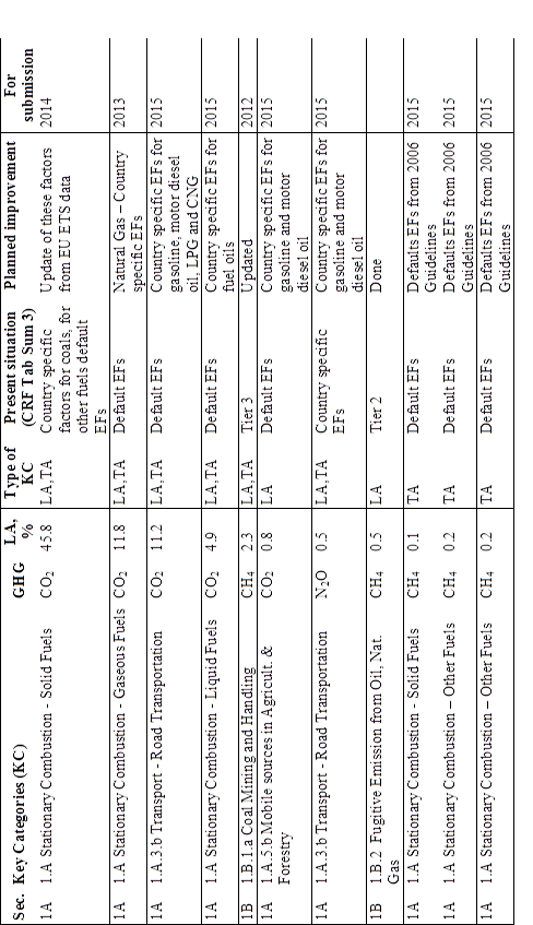
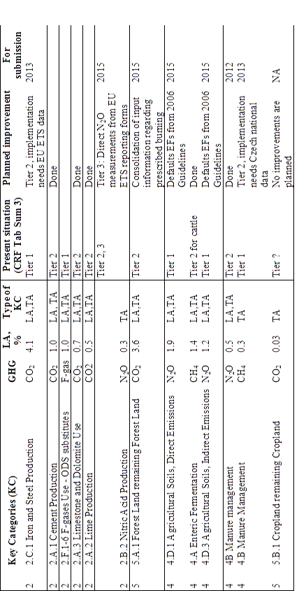
In addition to the planned introduction of the procedures of the higher Tiers in the individual sectors, the Improvement plan also includes a more general aspect. Here, it is planned to gradually refine the individual uncertainties in the emission factors and activity data in accordance with the ERT recommendations formulated in paragraph 37 of the expert review (ARR 2011). Substantial improvements should appear in the 2013 submission.

Specific suggestions for improvements in the individual sectors are described in the sections entitled “Source-specific planned improvements”, which are included in all the sector chapters.

[5] NEC - National Emission Ceilings according to Directive 2001/81/EC of the European Parliament and of the Council of 23 October 2001

^{^[6]}GHG emissions including emissions/removals from LULUCF

^{^[8]} (index form: 1990 = 100 for CO₂, CH₄ and N₂O and 1995 = 100 for HFCs, PFCs and SF₆)

[12] NEC - National Emission Ceilings according to Directive 2001/81/EC of the European Parliament and of the Council of 23 October 2001. Emissions targets for NO_x, NMVOC and SO₂ should be met by 2010

[13] A study performed solely for purposes of national GHG inventory

[14] Since 2009 the age limit for “Calves” shifted up to 8 months.

[15] Since 2009 the age limit for “Young bulls and heifers” shifted up to 8 -12 months.

[16] These parameters, together with the minimum width of 20 m for linear forest formations, were given in the Czech Initial Report under the Kyoto Protocol.

[17] The first cycle of the statistical (sample based, tree level) forest inventory was performed during 2001-2004 by the Forest Management Institute (FMI), Brandýs n. Labem. These data indicate significantly higher growing stock volumes (328 m³/ha under bark, excluding standing dead trees) than those reported so far for this country on the basis of data from forest management plans. This was mainly prescribed to methodological differences between the stand-wise inventory used for forest management planning and the tree-level, sample based statistical forest inventory (e.g., Černý et al. 2006; FMI 2007). However, only one inventory cycle of sample based inventory it is not readily usable for detecting carbon stock change in forests.

[18] The results of the CzechTerra national landscape inventory project show a mean growing stock volume of 305 m³/ha under bark (IFER 2010), i.e., significantly lower than the estimates of FMI (2007).

[19] Alternative approaches of the stock-change method (Eq. 3.2.3; IPCC 2003) were also analyzed (Cienciala et al. 2006a) for this category. However, for several reasons the default method was finally adopted, which is discussed in the cited study.

[20] Convention on Wetlands, Ramsar, Iran, 1971

[21] Based on the land-use history, the growth potential could be considered to be rather large. For example, as of 1990, the category included 50.7 th. ha of ponds, which represented only 28 % of their extent during the peak period in the 16^th Century (Marek 2002)

[22] Due to changes in the statistical data, we are no longer able to identify Pet. ref./Petrochemicals

[23] Amount of organic pollution associated with this technology is the average pollution per capita multiplied by the number of people not connected to sewers (
Tab. 8‑10)

[24] All references used in this chapter can be found in Chapter 10 of the NIR text.

Editors	Ondrej Minovsky (CHMI), coordinator of NIS Pavel Fott (CHMI)
Executive Summary	Ondrej Minovsky (CHMI)
Chapter 1 - Introduction and General Issues	Pavel Fott (CHMI) Ondrej Minovsky (CHMI)
Chapter 2 - Trend in Total Emissions	Ondrej Minovsky (CHMI)
Chapter 3 - Energy - (CRF sector 1)	Vladimir Neuzil (KONEKO) Eva Krtkova (CHMI) Jakub Tichý (CDV) Jiri Jedlicka (CDV)
Chapter 4 - Industrial Processes (CRF sector 2)	Pavel Fott (CHMI) Dusan Vacha (external coworker of CHMI)
Chapter 5 - Solvent and Other Product Use (CRF sector 3)	Ondrej Minovsky (CHMI)
Chapter 6 - Agriculture (CRF sector 4)	Zuzana Exnerova (IFER)
Chapter 7 - Land Use, Land-Use Change and Forestry (CRF sector 5)	Emil Cienciala (IFER) Jan Apltauer (IFER)
Chapter 8 - Waste (CFR sector 6)	Miroslav Havranek (CUEC)
Chapter 10 – Recalculations and Improvements	Ondrej Minovsky (CHMI) Pavel Fott (CHMI)
Chapter 11 - KP LULUCF	Emil Cienciala (IFER) Jan Apltauer (IFER)
Chapter 12 – Information on Accounting of Kyoto units	Miroslav Rehor (OTE) Michal Danhelka (MoE)
Chapter 13 – Information on Changes in National System	Ondrej Minovsky (CHMI)
Chapter 14 – Information on Changes in National Registry	Miroslav Rehor (OTE) Michal Danhelka (MoE)
Chapter 15 – Information on Minimization of Adverse Impacts	Michal Danhelka (MoE)

Year	Afforestation/Reforestation (AR, kha/year)					Deforestation (D, kha/year)
Year	C to F	G to F	W to F	S to F	Total	F to C	F to G	F to W	F to S	Total
1990	0.71	0.52	0.01	0.00	1.24	0.10	0.09	0.02	0.28	0.49
1991	0.40	0.12	0.00	0.02	0.54	0.28	0.35	0.07	0.17	0.87
1992	0.21	0.12	0.01	0.00	0.34	0.14	0.25	0.04	0.31	0.74
1993	0.09	0.12	0.01	0.18	0.39	0.19	0.07	0.02	0.55	0.82
1994	0.20	0.21	0.12	0.90	1.43	0.11	0.08	0.02	0.38	0.59
1995	0.31	0.36	0.02	0.47	1.16	0.15	0.08	0.02	0.27	0.52
1996	0.86	0.40	0.03	0.50	1.79	0.18	0.35	0.02	0.36	0.90
1997	0.31	0.43	0.04	0.90	1.69	0.23	0.17	0.04	0.37	0.80
1998	0.48	0.68	0.10	2.25	3.51	0.39	0.39	0.05	0.53	1.37
1999	0.33	0.45	0.04	0.72	1.54	0.12	0.08	0.05	0.60	0.84
2000	0.47	0.54	0.08	2.36	3.46	0.10	0.14	0.06	0.37	0.67
2001	0.44	0.49	0.04	1.15	2.12	0.07	0.08	0.02	0.33	0.49
2002	1.13	0.94	0.03	2.54	4.64	0.04	0.06	0.08	0.32	0.50
2003	0.70	0.57	0.03	0.72	2.02	0.08	0.14	0.05	0.52	0.78
2004	0.75	0.84	0.02	0.64	2.26	0.10	0.07	0.03	0.50	0.69
2005	0.86	0.90	0.01	0.58	2.35	0.10	0.09	0.03	0.43	0.66
2006	1.05	0.65	0.03	0.45	2.18	0.05	0.06	0.03	0.32	0.47
2007	0.92	0.58	0.02	0.92	2.45	0.02	0.07	0.02	0.26	0.38
2008	0.80	0.47	0.09	0.91	2.27	0.10	0.05	0.03	0.26	0.44
2009	0.78	0.67	0.09	1.10	2.65	0.04	0.11	0.03	0.28	0.47
2010	1.10	0.63	0.08	0.93	2.74	0.10	0.09	0.06	0.32	0.56

Year	Convention and KP LULUCF reporting categories and their areas (kha) since 1990
Year	Beech	Oak	Pine	Spruce	CA	5A2	5A	FLRFL	RA	FM
1990	372.1	152.4	455.4	1 503.8	40.6	52.6	2 576.9	2 524.3	51.4	2 575.7
1991	375.3	153.0	455.5	1 500.2	40.7	51.9	2 576.7	2 524.8	50.1	2 574.9
1992	378.7	154.2	454.3	1 500.3	41.9	47.1	2 576.5	2 529.4	45.0	2 574.4
1993	381.3	154.9	452.6	1 499.7	41.4	46.1	2 576.1	2 530.0	43.6	2 573.5
1994	384.9	155.0	450.9	1 502.1	39.8	44.2	2 576.9	2 532.8	40.2	2 573.0
1995	388.3	155.6	451.2	1 503.0	38.9	40.6	2 577.5	2 537.0	35.5	2 572.4
1996	391.0	157.3	450.5	1 502.0	38.1	39.5	2 578.4	2 538.9	32.6	2 571.5
1997	394.4	157.4	450.1	1 503.2	36.0	38.1	2 579.2	2 541.1	29.5	2 570.6
1998	400.9	157.8	452.8	1 499.1	33.7	36.8	2 581.1	2 544.3	24.7	2 569.1
1999	403.7	159.7	448.9	1 504.1	32.2	33.1	2 581.8	2 548.7	19.5	2 568.1
2000	408.1	161.8	447.7	1 503.6	31.0	32.4	2 584.5	2 552.1	15.3	2 567.5
2001	413.2	163.0	446.5	1 503.0	29.8	30.7	2 586.1	2 555.5	11.5	2 566.9
2002	419.0	164.5	444.5	1 499.2	28.3	34.6	2 590.2	2 555.6	10.7	2 566.3
2003	426.3	166.1	443.3	1 493.2	27.0	35.4	2 591.3	2 555.9	9.5	2 565.4
2004	431.9	166.9	440.9	1 489.8	26.8	36.6	2 592.8	2 556.3	8.4	2 564.7
2005	438.0	167.5	439.4	1 486.0	26.3	37.3	2 594.5	2 557.2	6.8	2 564.0
2006	442.4	169.4	437.6	1 482.9	25.9	37.9	2 596.2	2 558.2	5.3	2 563.5
2007	448.2	170.7	435.7	1 479.1	26.1	38.5	2 598.2	2 559.7	3.4	2 563.1
2008	455.2	173.0	433.9	1 471.9	27.1	38.9	2 600.0	2 561.1	1.5	2 562.6
2009	461.5	174.2	432.0	1 466.7	27.6	40.0	2 602.1	2 562.1	0.0	2 562.1
2010	465.9	176.2	430.8	1 461.6	28.1	41.5	2 604.2	2 562.7	0.0	2 561.5

Campaign Decay stage	NFI – ref. year 2003	CzechTerra – ref. year 2009
Wood is hard	7.47 (7.02 - 7.93)	9.54 (7.58 – 11.5)
Soft periphery, centre hard	3.75 (3.48 - 4.02)	5.10 (2.81 – 7.38)
Hard periphery, centre soft	0.82 (0.73 - 0.90)	1.28 (0.72 – 1.85)
Totally soft/rotten	6.28 (5.98 - 6.59)	4.79 (3.84 – 5.74)

Action	Implementation by the Party
(a) The progressive reduction or phasing out of market imperfections, fiscal incentives, tax and duty exemptions and subsidies in all greenhouse-gas-emitting sectors, taking into account the need for energy price reforms to reflect market prices and externalities.	The ongoing liberalization of energy market is in line with EU policies and directives. No significant market distortions have been identified. Consumption taxes for electricity and fossil fuels were harmonized recently. The main instrument addressing externalities is the emission trading under the EU ETS. Introduction of new instruments is subject to economic modelling and regulatory impact assessment.
(b) Removing subsidies associated with the use of environmentally unsound and unsafe technologies.	No subsidies for environmentally unsound and unsafe technologies have been identified.
(c) Cooperating in the technological development of non-energy uses of fossil fuels and supporting developing country Parties to this end.	The Czech Republic does not take part in any such activity.
(d) Cooperating in the development, diffusion, and transfer of less-greenhouse-gas-emitting advanced fossil-fuel technologies, and/or technologies, relating to fossil fuels, that capture and store greenhouse gases, and encouraging their wider use; and facilitating the participation of the least developed countries and other non-Annex I Parties in this effort.	Advanced low-carbon technologies are currently not a priority area in the Czech Republic’s research, development and innovation system. Research and development is focused on improving efficiency of currently available technologies. In 2009 and 2010 the project “Towards geological storage of CO₂ in the Czech Republic” (TOGEOS) was carried out. Resullts were published in article: D.G. Hatzignatiou, F. Riis, R. Berenblyum, V. Hladik, R. Lojka, J. Francu, Screening and evaluation of a saline aquifer for CO₂ storage: Central Bohemian Basin, Czech Republic, International Journal of Greenhouse Gas Control, Volume 5, Issue 6, November 2011. There is currently no ongoing or planned CCS programme or demonstration project in the Czech Republic.
(e) Strengthening the capacity of developing country Parties identified in Article 4, paragraphs 8 and 9, of the Convention for improving efficiency in upstream and downstream activities relating to fossil fuels, taking into consideration the need to improve the environmental efficiency of these activities.	The Czech Republic supports technology and capacity development through development assistance. Example of such activities is a project for modernization of powering and control of power plant block connected with establishment of a technical training centre at the University in Ulan Bator, Mongolia.
(f) Assisting developing country Parties which are highly dependent on the export and consumption of fossil fuels in diversifying their economies.	The Czech Republic is cooperating in several bilateral development assistance projects focusing on reduction of fossil fuels dependence and development of renewable energy sources, inter alia: - Increasing energy independence of remote regions in Georgia with solar thermal and photovoltaic systems - Construction of biomass heating plant and heat distribution network in Bosnia and Herzegovina - Development of biogas and photovoltaic energy sources in rural areas of Vietnam - Subsidizing biodigesters construction in rural areas of Cambodia to stimulate the emerging market - Development of small and medium size energy sources and interconnecting networks in Palestine

AACLC	Aggregate areas of cadastral land categories
APL	Association of Industrial Distilleries (Asociace průmyslových lihovarů)
ARR	Annual Review Report
AVNH	Association of Coatings Producers (Asociace výrobců nátěrových hmot)
AWMS	Animal Waste Management System
BOD	Biochemical Oxygen Demand
CAPPO	Czech Association of the Petroleum Industry (Česká asociace petrolejářského průmyslu a obchodu)
CCA	Czech Cement Association
CDV	Transport Research Centre (Centrum dopravního výzkumu)
CGA	Czech Gas Association
CNG	Compressed Natural Gas
COD	Chemical Oxygen Demand
COP	Conference of Parties
COSMC	Czech Office for Surveying, Mapping and Cadastre
COŽP UK	Centrum pro otázky životního prostředí Univerzity Karlovy
CUEC	Charles University Environment Center
CULS	Czech University of Life Sciences
CzSO	Czech Statistical Office
ČHMÚ	Český hydrometeorologický ústav
ČPS	Český plynárenský svaz
ČSÚ	Český statistický úřad
DOC	Degradable Organic Carbon
EEA	European Environmental Agency
EIG	Emission Inventory Guidebook
ERT	Expert Review Team
ETS	Emission Trading Scheme
FAO	Food and Agriculture Organization
FMI	Forest Management Institute, Brandýs nad Labem
FMP	Forest Management Plans
FOD (model)	First Order Decay (model)
GHG	Greenhouse Gas
HDV	Heavy Duty Vehicle
CHMI	Czech Hydrometeorological Institute
IEA	International Energy Agency
IFER	Institute of Forest Ecosystem Research (Ústav pro výzkum lesních ekosystémů)
IGU	International Gas Union
IPCC	Intergovernmental Panel of Climate Change
ISPOP	Integrovaný systém plnění ohlašovacích povinností
LDV	Light Duty Vehicle
LPG	Liquid Petroleum Gas
LTO	Landing/Taking-off
LULUCF	Land Use, Land-Use Change and Forestry
MA	Ministry of Agriculture (CR)
MCF	Methane Correction Factor
MIT	Ministry of Industry and Trade (CR)
MoE (CR)	Ministry of Environment (CR)
MPO	Ministerstvo průmyslu a obchodu (ČR)
MSW	Municipal Solid Waste
MZe	Ministerstvo zemědělství (ČR)
MŽP (ČR)	Ministerstvo životního prostředí (ČR)
NACE	Nomenclature Classification of Economic Activities
NIR	National Inventory System
NIS	National Inventory System (National system under Kyoto protocol, Art. 5)
OKD, a.s.	Ostravsko karvinské doly, akciová společnost (Ostrava – Karvina Mines)
OTE	Operátor trhu s elektřinou, a.s. (Electricity Market Operator)
PC	Passenger Car
QA/QC	Quality Assurance / Quality Control
RA	Reference Approach
REZZO	Register of Emissions and Sources of Air Pollution (Registr emisí a zdrojů znečišťování ovzduší)
SA	Sectoral Approach
SWDS	Solid Waste Disposal Sites
ÚHÚL	Ústav pro hospodářskou úpravu lesů
UNECE	United Nations Economic Commission for Europe (Evropská hospodářská komise OSN)
UNFCCC	United Nation Framework Convention on Climate Change
ÚVVP	Institute for Research and Use of Fuels (Ústav pro výzkum a využití paliv)
VŠCHT	Institute of Chemical Technology (Vysoká škola chemicko technologická)

Reference Approach [PJ]	Sectoral Approach [PJ]	Apparent energy consumption [PJ]	Difference [%]
1 925	1 708	1 744	2,14
1 772	1 641	1 639	-0,11
1 632	1 477	1 482	0,34
1 586	1 462	1 458	-0,29
1 510	1 348	1 377	2,21
1 535	1 386	1 411	1,84
1 594	1 448	1 468	1,44
1 604	1 414	1 479	4,57
1 539	1 349	1 406	4,25
1 422	1 296	1 307	0,86
1 526	1 382	1 405	1,69
1 553	1 401	1 433	2,25
1 526	1 364	1 400	2,62
1 547	1 395	1 410	1,12
1 565	1 412	1 413	0,03
1 547	1 427	1 404	-1,65
1 573	1 436	1 420	-1,10
1 573	1 424	1 424	-0,01
1 510	1 380	1 360	-1,44
1 390	1 310	1 271	-2,92
1 466	1 360	1 334	-1,89

Reference Approach [Gg]	Sectoral Approach [Gg]	Difference [%]
148 802	145 894	1,99
139 708	140 063	-0,25
125 563	124 432	0,91
122 857	123 371	-0,42
115 339	113 653	1,48
116 840	115 463	1,19
120 064	119 294	0,64
121 329	115 698	4,87
114 286	109 440	4,43
105 483	104 420	1,02
115 585	113 232	2,08
117 099	113 805	2,89
114 134	110 522	3,27
115 028	113 000	1,79
115 021	114 030	0,87
114 049	115 106	-0,92
115 404	115 807	-0,35
116 320	115 313	0,87
110 058	110 998	-0,85
102 961	105 726	-2,62
107 046	109 181	-1,96

SOLID FUELS	Coking Coal [kt/year]	Sub Bitumin. Coal [kt/year]	Lignite/Brown Coal [kt/year]	Coke Oven Coke [kt/year]	Coal Tar [kt/year]
Indigenous Production	6023	5 412	43 774	2 548	195
Total Imports (Balance)	909	1 073	58	885	276
Total Exports (Balance)	3499	2 772	1 056	875	10
International Marine Bunkers	0	0	0	0	0
Stock Changes (National Territory)	-64	702	956	52	2
Inland Consumption (Calculated)	3369	4 415	43 732	2 610	463
Statistical Differences	132	-264	-1 182	0	0
Transformation Sector	3237	3 882	40 732	2 078	20
Main Activity Producer Electricity Plants	0	1 237	26 176	0	0
Main Activity Producer CHP Plants	0	2 361	9 148	0	4
Main Activity Producer Heat Plants	0	54	210	1	3
Autoproducer Electricity Plants	0	0	416	0	0
Autoproducer CHP Plants	0	230	2 911	0	1
Autoproducer Heat Plants	0	0	22	0	0
Patent Fuel Plants (Transformation)	0	0	0	0	0
Coke Ovens (Transformation)	3237	0	0	73	0
BKB Plants (Transformation)	0	0	287	0	0
Gas Works (Transformation)	0	0	1 562	0	0
Blast Furnaces (Transformation)	0	0	0	2 004	12
Coal Liquefaction Plants (Transformation)	0	0	0	0	0
Non-specified (Transformation)	0	0	0	0	0
Energy Sector	0	0	1	0	50
Own Use in Electricity, CHP and Heat Plants	0	0	0	0	0
Coal Mines	0	0	1	0	0
Patent Fuel Plants (Energy)	0	0	0	0	0
Coke Ovens (Energy)	0	0	0	0	0
BKB Plants (Energy)	0	0	0	0	0
Gas Works (Energy)	0	0	0	0	50
Blast Furnaces (Energy)	0	0	0	0	0
Petroleum Refineries	0	0	0	0	0
Coal Liquefaction Plants (Energy)	0	0	0	0	0
Non-specified (Energy)	0	0	0	0	0
Distribution Losses	0	37	11	0	0
Total Final Consumption	0	760	4 170	532	393
Total Non-Energy Use	0	0	0	0	326
Final Energy Consumption	0	760	4 170	532	67
Industry Sector	0	654	2 871	498	67
Iron and Steel	0	257	63	449	35
Chemical (including Petrochemical)	0	175	2 338	0	13
Non-Ferrous Metals	0	0	0	6	0
Non-Metallic Minerals	0	183	40	28	19
Transport Equipment	0	0	30	0	0
Machinery	0	0	35	4	0
Mining and Quarrying	0	2	6	0	0
Food, Beverages and Tobacco	0	17	68	6	0
Paper, Pulp and Printing	0	17	239	0	0
Wood and Wood Products	0	0	2	0	0
Construction	0	1	29	5	0
Textiles and Leather	0	2	13	0	0
Non-specified (Industry)	0	0	8	0	0
Transport Sector	0	0	1	0	0
Other Sectors	0	106	1 298	34	0
Commercial and Public Services	0	4	59	7	0
Residential	0	100	1 200	25	0
Agriculture/Forestry	0	2	31	2	0
Fishing	0	0	0	0	0
Non-specified (Other)	0	0	8	0	0

SOLID FUELS	BKB-PB [kt/year]	Gas Works Gas [TJ/year]	Coke Oven Gas [TJ/year]	Blast Furnace Gas [TJ/year]	Oxygen Steel Furnace Gas [TJ/year]
Indigenous Production	145	19 402	20 144	21 795	21795
Total Imports (Balance)	149	0	0	0	0
Total Exports (Balance)	71	0	0	0	0
International Marine Bunkers	0	0	0	0	0
Stock Changes (National Territory)	-3	0	0	0	0
Inland Consumption (Calculated)	220	19 402	20 144	21 795	21795
Statistical Differences	9	1 145	0	0	0
Transformation Sector	3	18 152	5 190	8 883	8883
Main Activity Producer Electricity Plants	0	0	0	0	0
Main Activity Producer CHP Plants	0	0	4 995	8 307	8307
Main Activity Producer Heat Plants	0	0	0	0	0
Autoproducer Electricity Plants	0	107	0	0	0
Autoproducer CHP Plants	3	18 045	195	576	576
Autoproducer Heat Plants	0	0	0	0	0
Patent Fuel Plants (Transformation)	0	0	0	0	0
Coke Ovens (Transformation)	0	0	0	0	0
BKB Plants (Transformation)	0	0	0	0	0
Gas Works (Transformation)	0	0	0	0	0
Blast Furnaces (Transformation)	0	0	0	0	0
Coal Liquefaction Plants (Transformation)	0	0	0	0	0
Non-specified (Transformation)	0	0	0	0	0
Energy Sector	7	105	8 604	3 442	3442
Own Use in Electricity, CHP and Heat Plants	0	0	0	0	0
Coal Mines	0	105	0	0	0
Patent Fuel Plants (Energy)	0	0	0	0	0
Coke Ovens (Energy)	0	0	8 604	1 692	1692
BKB Plants (Energy)	7	0	0	0	0
Gas Works (Energy)	0	0	0	0	0
Blast Furnaces (Energy)	0	0	0	1 750	1750
Petroleum Refineries	0	0	0	0	0
Coal Liquefaction Plants (Energy)	0	0	0	0	0
Non-specified (Energy)	0	0	0	0	0
Distribution Losses	0	0	301	698	698
Total Final Consumption	201	0	6 049	8 772	8772
Total Non-Energy Use	0	0	0	0	0
Final Energy Consumption	201	0	6 049	8 772	8772
Industry Sector	1	0	6 049	8 772	8772
Iron and Steel	0	0	5 444	8 571	8571
Chemical (including Petrochemical)	0	0	0	0	0
Non-Ferrous Metals	0	0	0	0	0
Non-Metallic Minerals	1	0	85	0	0
Transport Equipment	0	0	0	0	0
Machinery	0	0	520	201	201
Mining and Quarrying	0	0	0	0	0
Food, Beverages and Tobacco	0	0	0	0	0
Paper, Pulp and Printing	0	0	0	0	0
Wood and Wood Products	0	0	0	0	0
Construction	0	0	0	0	0
Textiles and Leather	0	0	0	0	0
Non-specified (Industry)	0	0	0	0	0
Transport Sector	0	0	0	0	0
Other Sectors	200	0	0	0	0
Commercial and Public Services	0	0	0	0	0
Residential	200	0	0	0	0
Agriculture/Forestry	0	0	0	0	0
Fishing	0	0	0	0	0
Non-specified (Other)	0	0	0	0	0

LIQUID FUELS	Crude Oil [kt/year]	Refinery Feedstocks [kt/year]	Additives Oxygenates [kt/year]
Indigenous Production	176	0	96
From Other Sources	0	0	270
From Other Sources - Coal	0	0	0
From Other Sources - Natural Gas	0	0	0
From Other Sources - Renewables	0	0	270
Backflows to Refineries	0	78	0
Primary Product Receipts	0	0	0
Refinery Gross Output	0	0	0
Inputs of Recycled Products	0	0	0
Refinery Fuel	0	0	0
Total Imports (Balance)	7 727	0	33
Total Exports (Balance)	20	0	0
International Marine Bunkers	0	0	0
Interproduct Transfers	0	0	0
Products Transferred	0	142	0
Direct Use	0	0	121
Stock Changes (National Territory)	18	-2	3
Refinery Intake (Calculated)	7 901	218	281
Gross Inland Deliveries (Calculated)	0	0	0
Statistical Differences	0	0	0
Gross Inland Deliveries (Observed)	0	0	0
Refinery Intake (Observed)	7 901	218	281

LIQUID FUELS	Refinery Gas [kt/year]	LPG [kt/year]	Naphtha [kt/year]	Motor Gasoline [kt/year]	Biogasoline [kt/year]	Aviation Gasoline [kt/year]
Refinery Gross Output	155	215	860	1 509	46	0
Refinery Fuel	140	0	0	0	0	0
Total Imports (Balance)	0	69	70	591	12	2
Total Exports (Balance)	0	128	27	253	5	0
International Marine Bunkers	0	0	0	0	0	0
Stock Changes (National Territory)	0	3	14	-30	-4	0
Gross Inland Deliveries (Calculated)	15	186	917	1 858	90	2
Statistical Differences	0	1	0	0	0	0
Gross Inland Deliveries (Observed)	15	185	917	1 858	90	2
Refinery Intake (Observed)	0	0	0	0	0	0
Inland Demand (Total Consumption)	15	185	917	1 858	90	2
Transformation Sector	0	0	0	0	0	0
Main Activity Producer Electricity Plants	0	0	0	0	0	0
Autoproducer Electricity Plants	0	0	0	0	0	0
Main Activity Producer CHP Plants	0	0	0	0	0	0
Autoproducer CHP Plants	0	0	0	0	0	0
Main Activity Producer Heat Plants	0	0	0	0	0	0
Autoproducer Heat Plants	0	0	0	0	0	0
Gas Works (Transformation)	0	0	0	0	0	0
For Blended Natural Gas	0	0	0	0	0	0
Coke Ovens (Transformation)	0	0	0	0	0	0
Blast Furnaces (Transformation)	0	0	0	0	0	0
Petrochemical Industry	0	0	0	0	0	0
Patent Fuel Plants (Transformation)	0	0	0	0	0	0
Non-specified (Transformation)	0	0	0	0	0	0
Energy Sector	0	0	0	0	0	0
Coal Mines	0	0	0	0	0	0
Oil and Gas Extraction	0	0	0	0	0	0
Coke Ovens (Energy)	0	0	0	0	0	0
Blast Furnaces (Energy)	0	0	0	0	0	0
Gas Works (Energy)	0	0	0	0	0	0
Own Use in Electricity, CHP and Heat Plants	0	0	0	0	0	0
Non-specified (Energy)	0	0	0	0	0	0
Distribution Losses	0	0	0	0	0	0
Total Final Consumption	15	185	917	1 858	90	2
Transport Sector	0	76	0	1 858	90	2
International Aviation	0	0	0	0	0	0
Domestic Aviation	0	0	0	0	0	2
Road	0	76	0	1 858	90	0
Rail	0	0	0	0	0	0
Domestic Navigation	0	0	0	0	0	0
Pipeline Transport	0	0	0	0	0	0
Non-specified (Transport)	0	0	0	0	0	0
Industry Sector	15	102	917	0	0	0
Iron and Steel	0	0	0	0	0	0
Chemical (including Petrochemical)	15	96	917	0	0	0
Non-Ferrous Metals	0	0	0	0	0	0
Non-Metallic Minerals	0	1	0	0	0	0
Transport Equipment	0	1	0	0	0	0
Machinery	0	1	0	0	0	0
Mining and Quarrying	0	0	0	0	0	0
Food, Beverages and Tobacco	0	1	0	0	0	0
Paper, Pulp and Printing	0	0	0	0	0	0
Wood and Wood Products	0	0	0	0	0	0
Construction	0	1	0	0	0	0
Textiles and Leather	0	1	0	0	0	0
Non-specified (Industry)	0	0	0	0	0	0
Other Sectors	0	7	0	0	0	0
Commercial and Public Services	0	1	0	0	0	0
Residential	0	4	0	0	0	0
Agriculture/Forestry	0	2	0	0	0	0
Fishing	0	0	0	0	0	0
Non-specified (Other)	0	0	0	0	0	0
Total Non-Energy Use	15	96	917	0	0	0
Non-Energy Use in Transformation Sector	0	0	0	0	0	0
Non-Energy Use in Energy Sector	0	0	0	0	0	0
Non-Energy Use in Transport	0	0	0	0	0	0
Non-Energy Use in Industry	15	96	917	0	0	0
Of which: Non-Energy Use-Chemical/Petrochem	15	96	917	0	0	0
Non-Energy Use in Other Sectors	0	0	0	0	0	0

LIQUID FUELS	Kerosene Type Jet Fuel [kt/year]	Other Kerosene [kt/year]	Transport Diesel [kt/year]	Biodiesel [kt/year]	Heating and Other Gasoil [kt/year]	Residual Fuel Oil [kt/year]
Refinery Gross Output	144	0	3 310	103	70	239
Refinery Fuel	0	0	0	0	0	13
Total Imports (Balance)	205	3	1 237	27	12	72
Total Exports (Balance)	0	0	700	15	15	77
International Marine Bunkers	0	0	0	0	0	0
Stock Changes (National Territory)	-7	0	77	1	0	-9
Gross Inland Deliveries (Calculated)	330	3	3 980	196	91	224
Statistical Differences	0	0	0	0	0	0
Gross Inland Deliveries (Observed)	330	3	3 980	196	91	224
Refinery Intake (Observed)	0	0	0	0	0	0
Inland Demand (Total Consumption)	330	3	3 980	196	91	224
Transformation Sector	0	0	0	0	3	101
Main Activity Producer Electricity Plants	0	0	0	0	0	7
Autoproducer Electricity Plants	0	0	0	0	0	0
Main Activity Producer CHP Plants	0	0	0	0	1	34
Autoproducer CHP Plants	0	0	0	0	0	40
Main Activity Producer Heat Plants	0	0	0	0	2	18
Autoproducer Heat Plants	0	0	0	0	0	2
Gas Works (Transformation)	0	0	0	0	0	0
For Blended Natural Gas	0	0	0	0	0	0
Coke Ovens (Transformation)	0	0	0	0	0	0
Blast Furnaces (Transformation)	0	0	0	0	0	0
Petrochemical Industry	0	0	0	0	0	0
Patent Fuel Plants (Transformation)	0	0	0	0	0	0
Non-specified (Transformation)	0	0	0	0	0	0
Energy Sector	0	0	14	0	3	0
Coal Mines	0	0	14	0	0	0
Oil and Gas Extraction	0	0	0	0	0	0
Coke Ovens (Energy)	0	0	0	0	0	0
Blast Furnaces (Energy)	0	0	0	0	0	0
Gas Works (Energy)	0	0	0	0	0	0
Own Use in Electricity, CHP and Heat Plants	0	0	0	0	0	0
Non-specified (Energy)	0	0	0	0	3	0
Distribution Losses	0	0	0	0	0	0
Total Final Consumption	330	3	3 966	196	85	123
Transport Sector	330	0	3 593	196	0	0
International Aviation	303	0	0	0	0	0
Domestic Aviation	27	0	0	0	0	0
Road	0	0	3 497	196	0	0
Rail	0	0	92	0	0	0
Domestic Navigation	0	0	4	0	0	0
Pipeline Transport	0	0	0	0	0	0
Non-specified (Transport)	0	0	0	0	0	0
Industry Sector	0	0	48	0	72	117
Iron and Steel	0	0	0	0	0	26
Chemical (including Petrochemical)	0	0	0	0	25	32
Non-Ferrous Metals	0	0	0	0	0	0
Non-Metallic Minerals	0	0	0	0	1	13
Transport Equipment	0	0	0	0	1	0
Machinery	0	0	0	0	2	2
Mining and Quarrying	0	0	0	0	0	0
Food, Beverages and Tobacco	0	0	0	0	1	15
Paper, Pulp and Printing	0	0	0	0	0	14
Wood and Wood Products	0	0	0	0	1	5
Construction	0	0	46	0	3	3
Textiles and Leather	0	0	0	0	0	3
Non-specified (Industry)	0	0	2	0	38	4
Other Sectors	0	3	325	0	13	6
Commercial and Public Services	0	0	3	0	4	3
Residential	0	0	0	0	0	0
Agriculture/Forestry	0	0	313	0	5	3
Fishing	0	0	0	0	0	0
Non-specified (Other)	0	3	9	0	4	0
Total Non-Energy Use	0	0	0	0	25	0
Non-Energy Use in Transformation Sector	0	0	0	0	0	0
Non-Energy Use in Energy Sector	0	0	0	0	0	0
Non-Energy Use in Transport	0	0	0	0	0	0
Non-Energy Use in Industry	0	0	0	0	25	0
Of which: Non-Energy Use-Chemical/Petrochem	0	0	0	0	25	0
Non-Energy Use in Other Sectors	0	0	0	0	0	0

LIQUID FUELS	White Spirit SBP [kt/year]	Lubricants [kt/year]	Bitumen [kt/year]	Paraffin Wax [kt/year]	Petroleum Coke [kt/year]	Other Products [kt/year]
Refinery Gross Output	0	172	523	9	0	1 117
Refinery Fuel	0	0	0	0	0	88
Total Imports (Balance)	15	117	213	13	7	107
Total Exports (Balance)	3	65	309	7	2	28
International Marine Bunkers	0	0	0	0	0	0
Stock Changes (National Territory)	0	-3	1	0	0	-30
Gross Inland Deliveries (Calculated)	12	158	428	15	5	984
Statistical Differences	0	0	0	0	0	0
Gross Inland Deliveries (Observed)	12	158	428	15	5	984
Refinery Intake (Observed)	0	0	0	0	0	0
Inland Demand (Total Consumption)	12	158	428	15	5	984
Transformation Sector	0	0	0	0	0	78
Main Activity Producer Electricity Plants	0	0	0	0	0	0
Autoproducer Electricity Plants	0	0	0	0	0	0
Main Activity Producer CHP Plants	0	0	0	0	0	0
Autoproducer CHP Plants	0	0	0	0	0	0
Main Activity Producer Heat Plants	0	0	0	0	0	0
Autoproducer Heat Plants	0	0	0	0	0	0
Gas Works (Transformation)	0	0	0	0	0	0
For Blended Natural Gas	0	0	0	0	0	0
Coke Ovens (Transformation)	0	0	0	0	0	0
Blast Furnaces (Transformation)	0	0	0	0	0	0
Petrochemical Industry	0	0	0	0	0	78
Patent Fuel Plants (Transformation)	0	0	0	0	0	0
Non-specified (Transformation)	0	0	0	0	0	0
Energy Sector	0	0	0	0	0	0
Coal Mines	0	0	0	0	0	0
Oil and Gas Extraction	0	0	0	0	0	0
Coke Ovens (Energy)	0	0	0	0	0	0
Blast Furnaces (Energy)	0	0	0	0	0	0
Gas Works (Energy)	0	0	0	0	0	0
Own Use in Electricity, CHP and Heat Plants	0	0	0	0	0	0
Non-specified (Energy)	0	0	0	0	0	0
Distribution Losses	0	0	0	0	0	0
Total Final Consumption	12	158	428	15	5	906
Transport Sector	0	151	0	0	0	0
International Aviation	0	0	0	0	0	0
Domestic Aviation	0	0	0	0	0	0
Road	0	141	0	0	0	0
Rail	0	10	0	0	0	0
Domestic Navigation	0	0	0	0	0	0
Pipeline Transport	0	0	0	0	0	0
Non-specified (Transport)	0	0	0	0	0	0
Industry Sector	12	7	426	15	5	906
Iron and Steel	0	0	0	0	0	2
Chemical (including Petrochemical)	1	0	0	0	0	643
Non-Ferrous Metals	0	0	0	0	0	0
Non-Metallic Minerals	0	0	0	0	0	16
Transport Equipment	0	0	0	0	0	0
Machinery	0	0	0	0	5	0
Mining and Quarrying	0	0	0	0	0	3
Food, Beverages and Tobacco	0	0	0	0	0	1
Paper, Pulp and Printing	0	0	0	0	0	0
Wood and Wood Products	0	0	0	0	0	1
Construction	0	0	426	0	0	5
Textiles and Leather	0	0	0	0	0	0
Non-specified (Industry)	11	7	0	15	0	235
Other Sectors	0	0	2	0	0	0
Commercial and Public Services	0	0	0	0	0	0
Residential	0	0	0	0	0	0
Agriculture/Forestry	0	0	0	0	0	0
Fishing	0	0	0	0	0	0
Non-specified (Other)	0	0	2	0	0	0
Total Non-Energy Use	12	0	426	15	0	721
Non-Energy Use in Transformation Sector	0	0	0	0	0	78
Non-Energy Use in Energy Sector	0	0	0	0	0	0
Non-Energy Use in Transport	0	0	0	0	0	0
Non-Energy Use in Industry	12	0	426	15	0	643
Of which: Non-Energy Use-Chemical/Petrochem	0	0	0	0	0	643
Non-Energy Use in Other Sectors	0	0	0	0	0	0

Indigenous Production	7 779
Associated Gas	5 308
Non-Associated Gas	2 471
Colliery Gas	0
From Other Sources	0
Total Imports (Balance)	324 541
Total Exports (Balance)	6 063
International Marine Bunkers	0
Stock Changes (National Territory)	47 476
Inland Consumption (Calculated)	373 733
Statistical Differences	19 778
Inland Consumption (Observed)	353 955
Recoverable Gas
Opening Stock Level (National Territory)	105 035
Closing Stock Level (National Territory)	57 559
Memo:
Gas Vented	0
Gas Flared	0
Memo: Cushion Gas
Cushion Gas Closing Stock Level	0
Memo: From other sources
From Other Sources - Oil	0
From Other Sources - Coal	0
From Other Sources - Renewables	0

Transformation Sector	47 708
Main Activity Producer Electricity Plants	649
Autoproducer Electricity Plants	0
Main Activity Producer CHP Plants	13 305
Autoproducer CHP Plants	4 875
Main Activity Producer Heat Plants	25 649
Autoproducer Heat Plants	3 230
Gas Works (Transformation)	0
Coke Ovens (Transformation)	0
Blast Furnaces (Transformation)	0
Gas-to-Liquids (GTL) Plants (Transformation)	0
Non-specified (Transformation)	0
Energy Sector	4 568
Coal Mines	0
Oil and Gas Extraction	156
Petroleum Refineries	4 412
Coke Ovens (Energy)	0
Blast Furnaces (Energy)	0
Gas Works (Energy)	0
Own Use in Electricity, CHP and Heat Plants	0
Liquefaction (LNG) / Regasification Plants	0
Gas-to-Liquids (GTL) Plants (Energy)	0
Non-specified (Energy)	0
Distribution Losses	5 606
Transport Sector	3 443
Road	402
of which Biogas	0
Pipeline Transport	3 041
Non-specified (Transport)	0
Industry Sector	106 134
Iron and Steel	13 250
Chemical (including Petrochemical)	11 564
Non-Ferrous Metals	1 880
Non-Metallic Minerals	24 801
Transport Equipment	7 846
Machinery	13 787
Mining and Quarrying	2 575
Food, Beverages and Tobacco	13 960
Paper, Pulp and Printing	4 544
Wood and Wood Products	1 466
Construction	3 558
Textiles and Leather	2 270
Non-specified (Industry)	4 633
Other Sectors	181 950
Commercial and Public Services	64 120
Residential	110 828
Agriculture/Forestry	2 972
Fishing	0
Non-specified (Other)	4 030