XII. CREATION OF AMBIENT AIR POLLUTION MAPS

Directive No. 2008/50/EC on ambient air quality and cleaner air for Europe, implemented in the Czech legislation (i.a. Decree No. 330/2012 Coll.), requires that air quality should be assessed in all zones and agglomerations throughout the territory of each member state. It further requires that fixed measurements should be used as a primary source of information for such assessment. The measured concentrations may be supplemented by modelling techniques and by indicative measurements, so that the resulting estimate provides adequate information on the spatial distribution of ambient air pollutant concentrations. The requirement to use fixed measurements as the primary source of information particularly pertains to areas in which pollutant concentrations exceed the upper assessment threshold. In order to retain a unified mapping methodology, this requirement is applied for the whole territory of the Czech Republic.

Therefore, concentrations of ambient air pollutants measured at individual measuring stations are the fundamental source of data for the creation of maps. The number of measuring stations is limited. In addition to measured (primary) data, the mapping procedure uses also various supplementary (secondary) data providing complex information about the whole territory while at the same time showing a regression relationship with the measured data. The main secondary source of information is represented by models of chemical transport and dispersion of pollutants, based on data from emission inventories and on meteorological data. In the Czech Republic, mainly the Eulerian chemical dispersion model CAMx is used, supplemented also by the Gaussian model SYMOS and the European Eulerian model EMEP. Furthermore, for individual pollutants, information on altitude or population density is used, for example (see Annex I for details). When combining the primary and secondary data, both the accuracy of the primary measured data and the complete coverage of the whole territory with the secondary data are utilised. The maps created regularly for the yearbook are based on the linear regression model followed by spatial interpolation of its residuals. As concerns interpolation methods, kriging and IDW are applied (see Annex I for details).

Urban and rural ambient air pollution differs in character. Urban air pollution is, due to the impact of emissions, generally higher than air pollution in rural areas. There is one exception, however, namely air pollution caused by ground-level ozone, for which the opposite is true. Urban and rural maps are therefore constructed separately, and the final map is produced by merging the urban map and the rural map using the grid of population density. For several pollutants (see Annex I), also the traffic layer is taken into consideration, in addition to the urban and rural layers. This layer is merged with the urban and rural background layers using the grid of traffic emissions. For the construction of the rural map, air pollution data measured at rural background stations are used as primary data. In the case of the urban map, air pollution data from urban and suburban background stations are used. For the potential traffic layer, data from traffic stations are used. The mapping procedure uses the classification of individual stations according to the AQIS database.

The maps are created using geographic information systems (GIS). The main source of data is the AQIS relational database of measured data on air pollution concentrations and the chemical composition of atmospheric precipitation. The maps are constructed with a spatial resolution of 1×1 km, using the Gauss-Krüger projection. The detailed specification of the mapping procedure for individual pollutants is presented in Annex I.

Since 1994 the DMÚ 200, DMR-2, DMÚ 25 and later the ZABAGED digital layers have been used to create the basic geographical and thematic layers in a standardized projection (Gauss-Krüger conformal projection). In recent years the latest layers of administrative division are created on the basis of materials provided by the CSO.

Mapping of rural and urban (and potential traffic) layers

The maps of rural and urban background pollution (and the potential pollution caused by traffic) are produced separately. They are constructed by combining primary (measured) data and secondary (model and further supplementary) data, see Horálek et al. (2007). The method used in this process is the linear regression model followed by spatial interpolation of its residuals. This method enables the use of supplementary data for the whole mapped territory. In cases when there are no suitable supplementary data, simple interpolation of the measured data is used. The estimate is calculated according to the following relation:

    (1)

where

                    is the estimated value of the concentration in the point s₀,
        X_i(s)            are various supplementary parameters in the point s₀ for i = 1, 2, …p,
        c, a₁, a₂,…   are the parameters of the linear regression model,
        h(s₀)           is the spatial interpolated value of the residuals of the linear regression model in the point s₀, calculated on the basis of the residuals in the points of measurement.

The spatial interpolation is carried out using the inverse distance weighting method (IDW) or using ordinary kriging (specifications for individual pollutants – in the Annex I). The IDW method is a simple deterministic method, where the weight of individual measuring stations in the interpolation depends only on their distance from the estimated point. Kriging, on the contrary, is a more advanced geostatistical method taking into account the structure of the air pollution field. However, the advantage of the IDW method consists in respecting the measured values in the points of measuring stations. Kriging does not generally respect the measured values. There is a solution, however, which is interpolation with the use of kriging, followed by the application of IDW on its residuals in the points of measurement.

Interpolation of residuals using IDW is calculated according to the relation: 

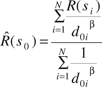         (2)

where
            is the estimate of the field of residuals in the point s₀,
         R(s_i)   is the residual of linear regression model in the point of measurement s_i, 
         N       is the number of surrounding stations used in interpolation,
         d_0i     is the distance between points s₀ and s_i,
         b       is the weight.

 

In ordinary kriging the interpolation of residuals is calculated according to the relation:


   při         (3)

where
        l₁, …,l_N     are the weights estimated on the basis of fitted variogram (see below),
        R(s_i)           is the residual of linear regression model in the point of measurement s_i.

The variogram describes the dependence of the between-points variability on the mutual distance of points, it is a measure of a spatial correlation (see e.g. Cressie 1993). The variogram is estimated by fitting spherical function in empirical variogram, calculated according to the relation:
 

,        (4)
 

where

                  is the empirical variogram of the field of residuals,
R(s_i), R(s_j)    are the residuals in the points of measurement s_i and s_j,
d_ij               is the distance of points s_i and s_j,
n                is the number of station couples s_i and s_j, with their mutual distance h±d,
d                 is the tolerance.

Spherical function and variogram parameters range, nugget and sill are illustrated in Fig. XII.1.

The calculated urban and rural (and potential traffic) layers are subsequently merged.

The merging of urban and rural (and potential traffic) layers

For the merging of the urban and rural layers the layer of population density is used, see e.g. Horálek et al. (2007), De Smet et al. (2011). The merging is carried out according to the relation:
 

                                                                  for    

                             for             (5)

                                                                           for     
 

where

                        is the result estimate of the concentration in the point s₀,
             is the concentration in the point s₀ for the rural or urban map,
        a(s₀)               is the population density in the point s₀,
        a₁, a₂              are classification intervals of the respective population density (see the Annex I).

 

The whole conception of separate mapping of ambient air pollution in rural and urban areas is based on the assumption that   for all common pollutants with the exception of ozone, or    or ozone. For the areas where this assumption is not fulfilled the layer created similarly as the urban and rural layers is used, nevertheless it is created on the basis of all background stations, without making the difference between the urban and the rural ones.

If also air pollution caused by traffic is mapped for the given pollutant, the traffic layer is added to the background (merged urban and rural) layer using the grid of traffic emissions:

                                                                  for  


             for            (6)

                                                        for  
 

where
            is the result estimate of the concentration in the point s₀,
            is the concentration in the point s₀ for the background layer,
            is the concentration in the point s₀ for the traffic layer,
        t(s₀)     are traffic emissions in the point s₀,
        t₁, t₂   

are the classification intervals of the respective traffic emissions (see the Annex I).

The above function is based on the assumption that   for common pollutants with the exception of ozone, or for ozone. For the areas where this assumption is not fulfilled the background layera is used.

 

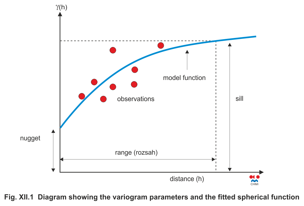
Fig. XII.1 Diagram showing the variogram parameters and the fitted spherical functions